
Chapter 3
FORWARD KINEMATICS:
THE
DENAVIT-HARTENBERG
CONVENTION
In this chapter we develop the forward or configuration kinematic equa-
tions for rigid robots. The forward kinematics problem is concerned with
the relationship between the individual joints of the robot manipulator and
the position and orientation of the tool or end-effector. Stated more formally,
the forward kinematics problem is to determine the position and orientation
of the end-effector, given the values for the joint variables of the robot. The
joint variables are the angles between the links in the case of revolute or
rotational joints, and the link extension in the case of prismatic or sliding
joints. The forward kinematics problem is to be contrasted with the inverse
kinematics problem, which will be studied in the next chapter, and which
is concerned with determining values for the joint variables that achieve a
desired position and orientation for the end-effector of the robot.
3.1
Kinematic Chains
As described in Chapter 1, a robot manipulator is composed of a set of
links connected together by various joints. The joints can either be very
simple, such as a revolute joint or a prismatic joint, or else they can be more
complex, such as a ball and socket joint. (Recall that a revolute joint is like
71

72CHAPTER 3. FORWARD KINEMATICS: THE DENAVIT-HARTENBERG CONVENTION
a hinge and allows a relative rotation about a single axis, and a prismatic
joint permits a linear motion along a single axis, namely an extension or
retraction.) The difference between the two situations is that, in the first
instance, the joint has only a single degree-of-freedom of motion: the angle of
rotation in the case of a revolute joint, and the amount of linear displacement
in the case of a prismatic joint. In contrast, a ball and socket joint has two
degrees-of-freedom. In this book it is assumed throughout that all joints
have only a single degree-of-freedom. Note that the assumption does not
involve any real loss of generality, since joints such as a ball and socket joint
(two degrees-of-freedom) or a spherical wrist (three degrees-of-freedom) can
always be thought of as a succession of single degree-of-freedom joints with
links of length zero in between.
With the assumption that each joint has a single degree-of-freedom, the
action of each joint can be described by a single real number: the angle of
rotation in the case of a revolute joint or the displacement in the case of a
prismatic joint. The objective of forward kinematic analysis is to determine
the cumulative effect of the entire set of joint variables. In this chapter
we will develop a set of conventions that provide a systematic procedure
for performing this analysis. It is, of course, possible to carry out forward
kinematics analysis even without respecting these conventions, as we did
for the two-link planar manipulator example in Chapter 1. However, the
kinematic analysis of an n-link manipulator can be extremely complex and
the conventions introduced below simplify the analysis considerably. More-
over, they give rise to a universal language with which robot engineers can
communicate.
A robot manipulator with n joints will have n + 1 links, since each joint
connects two links. We number the joints from 1 to n, and we number the
links from 0 to n, starting from the base. By this convention, joint i connects
link i − 1 to link i. We will consider the location of joint i to be fixed with
respect to link i − 1. When joint i is actuated, link i moves. Therefore, link
0 (the first link) is fixed, and does not move when the joints are actuated.
Of course the robot manipulator could itself be mobile (e.g., it could be
mounted on a mobile platform or on an autonomous vehicle), but we will
not consider this case in the present chapter, since it can be handled easily
by slightly extending the techniques presented here.
With the i
th
joint, we associate a joint variable, denoted by q
i
. In the
case of a revolute joint, q
i
is the angle of rotation, and in the case of a
3.1. KINEMATIC CHAINS
73
θ
1
θ
3
θ
2
z
2
z
3
x
0
z
0
x
1
x
2
x
3
y
3
z
1
y
1
y
2
y
0
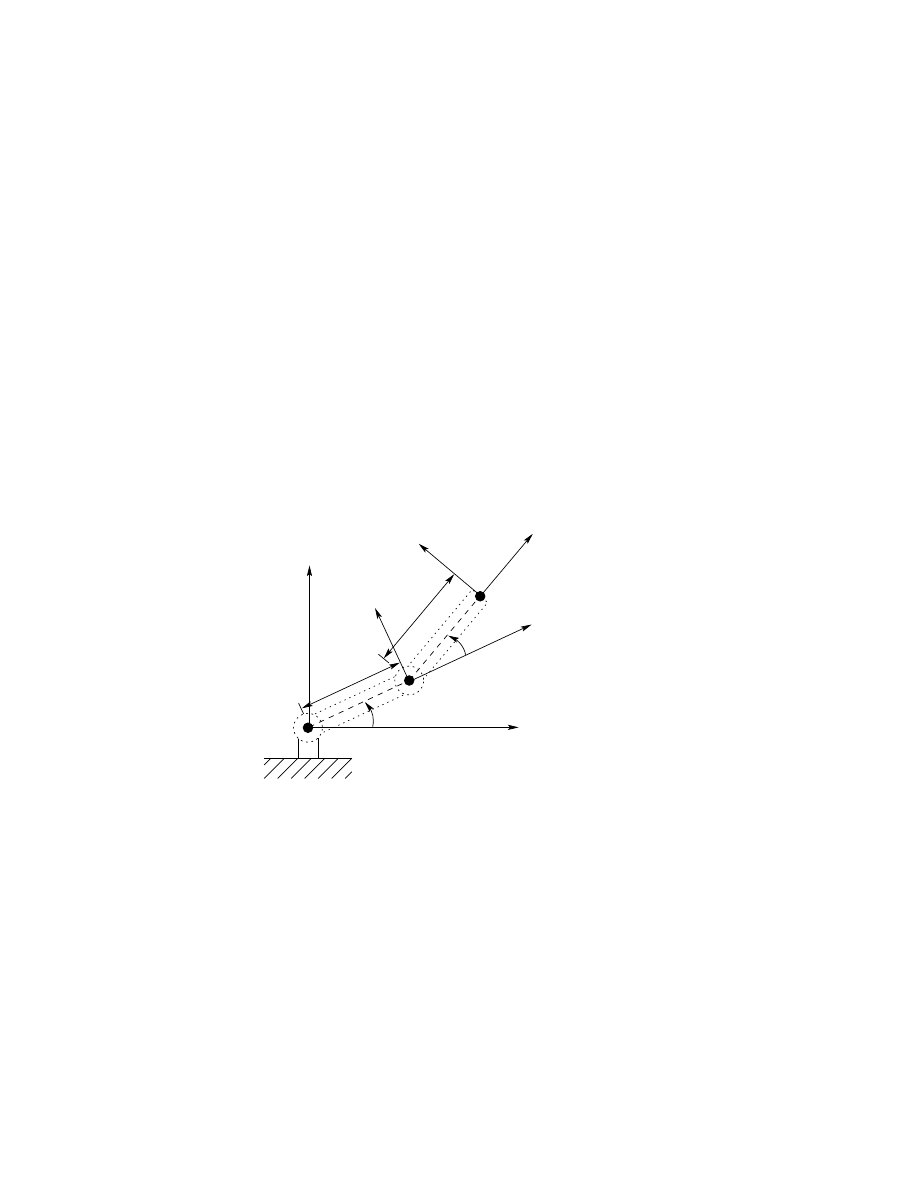
Figure 3.1: Coordinate frames attached to elbow manipulator.
prismatic joint, q
i
is the joint displacement:
q
i
=
(
θ
i
: joint i revolute
d
i
: joint i prismatic
.
(3.1)
To perform the kinematic analysis, we rigidly attach a coordinate frame
to each link. In particular, we attach o
i
x
i
y
i
z
i
to link i. This means that,
whatever motion the robot executes, the coordinates of each point on link
i
are constant when expressed in the i
th
coordinate frame. Furthermore,
when joint i is actuated, link i and its attached frame, o
i
x
i
y
i
z
i
, experience
a resulting motion. The frame o
0
x
0
y
0
z
0
, which is attached to the robot
base, is referred to as the inertial frame. Figure 3.1 illustrates the idea of
attaching frames rigidly to links in the case of an elbow manipulator.
Now suppose A
i
is the homogeneous transformation matrix that ex-
presses the position and orientation of o
i
x
i
y
i
z
i
with respect to o
i−1
x
i−1
y
i−1
z
i−1
.
The matrix A
i
is not constant, but varies as the configuration of the robot
is changed. However, the assumption that all joints are either revolute or
prismatic means that A
i
is a function of only a single joint variable, namely
q
i
. In other words,
A
i
= A
i
(q
i
).
(3.2)
Now the homogeneous transformation matrix that expresses the position
and orientation of o
j
x
j
y
j
z
j
with respect to o
i
x
i
y
i
z
i
is called, by convention,
a transformation matrix, and is denoted by T
i
j
. From Chapter 2 we see
that
T
i
j
= A
i+1
A
i+2
. . . A
j−1
A
j
if i < j

74CHAPTER 3. FORWARD KINEMATICS: THE DENAVIT-HARTENBERG CONVENTION
T
i
j
= I if i = j
(3.3)
T
i
j
= (T
j
i
)
−1
if j > i.
By the manner in which we have rigidly attached the various frames
to the corresponding links, it follows that the position of any point on the
end-effector, when expressed in frame n, is a constant independent of the
configuration of the robot. Denote the position and orientation of the end-
effector with respect to the inertial or base frame by a three-vector O
0
n
(which gives the coordinates of the origin of the end-effector frame with
respect to the base frame) and the 3 × 3 rotation matrix R
0
n
, and define the
homogeneous transformation matrix
H
=
"
R
0
n
O
0
n
0
1
#
.
(3.4)
Then the position and orientation of the end-effector in the inertial frame
are given by
H
= T
0
n
= A
1
(q
1
) · · · A
n
(q
n
).
(3.5)
Each homogeneous transformation A
i
is of the form
A
i
=
"
R
i−1
i
O
i−1
i
0
1
#
.
(3.6)
Hence
T
i
j
= A
i+1
· · · A
j
=
"
R
i
j
O
i
j
0
1
#
.
(3.7)
The matrix R
i
j
expresses the orientation of o
j
x
j
y
j
z
j
relative to o
i
x
i
y
i
z
i
and is given by the rotational parts of the A-matrices as
R
i
j
= R
i
i+1
· · · R
j−1
j
.
(3.8)
The coordinate vectors O
i
j
are given recursively by the formula
O
i
j
= O
i
j−1
+ R
i
j−1
O
j−1
j
,
(3.9)
These expressions will be useful in Chapter 5 when we study Jacobian ma-
trices.
In principle, that is all there is to forward kinematics! Determine the
functions A
i
(q
i
), and multiply them together as needed. However, it is pos-
sible to achieve a considerable amount of streamlining and simplification by
introducing further conventions, such as the Denavit-Hartenberg represen-
tation of a joint, and this is the objective of the remainder of the chapter.

3.2. DENAVIT HARTENBERG REPRESENTATION
75
3.2
Denavit Hartenberg Representation
While it is possible to carry out all of the analysis in this chapter using an
arbitrary frame attached to each link, it is helpful to be systematic in the
choice of these frames. A commonly used convention for selecting frames of
reference in robotic applications is the Denavit-Hartenberg, or D-H conven-
tion. In this convention, each homogeneous transformation A
i
is represented
as a product of four basic transformations
A
i
= R
z,θi
Trans
z,d
i
Trans
x,a
i
R
x,αi
(3.10)
=
c
θ
i
−s
θ
i
0 0
s
θ
i
c
θ
i
0 0
0
0
1 0
0
0
0 1
1 0 0
0
0 1 0
0
0 0 1 d
i
0 0 0
1
1 0 0 a
i
0 1 0
0
0 0 1
0
0 0 0
1
1
0
0
0
0 c
α
i
−s
α
i
0
0 s
α
i
c
α
i
0
0
0
0
1
=
c
θ
i
−s
θ
i
c
α
i
s
θ
i
s
α
i
a
i
c
θ
i
s
θ
i
c
θ
i
c
α
i
−c
θ
i
s
α
i
a
i
s
θ
i
0
s
α
i
c
α
i
d
i
0
0
0
1
where the four quantities θ
i
, a
i
, d
i
, α
i
are parameters associated with link
i
and joint i. The four parameters a
i
, α
i
, d
i
, and θ
i
in (3.10) are generally
given the names link length, link twist, link offset, and joint angle,
respectively. These names derive from specific aspects of the geometric
relationship between two coordinate frames, as will become apparent below.
Since the matrix A
i
is a function of a single variable, it turns out that three
of the above four quantities are constant for a given link, while the fourth
parameter, θ
i
for a revolute joint and d
i
for a prismatic joint, is the joint
variable.
From Chapter 2 one can see that an arbitrary homogeneous transforma-
tion matrix can be characterized by six numbers, such as, for example, three
numbers to specify the fourth column of the matrix and three Euler angles
to specify the upper left 3 × 3 rotation matrix. In the D-H representation, in
contrast, there are only four parameters. How is this possible? The answer
is that, while frame i is required to be rigidly attached to link i, we have
considerable freedom in choosing the origin and the coordinate axes of the
frame. For example, it is not necessary that the origin, O
i
, of frame i be
placed at the physical end of link i. In fact, it is not even necessary that
frame i be placed within the physical link; frame i could lie in free space —
so long as frame i is rigidly attached to link i. By a clever choice of the origin
and the coordinate axes, it is possible to cut down the number of parameters
76CHAPTER 3. FORWARD KINEMATICS: THE DENAVIT-HARTENBERG CONVENTION
z
0
x
1
y
1
α
x
0
θ
a
d
z
1
y
0
O
0
O
1
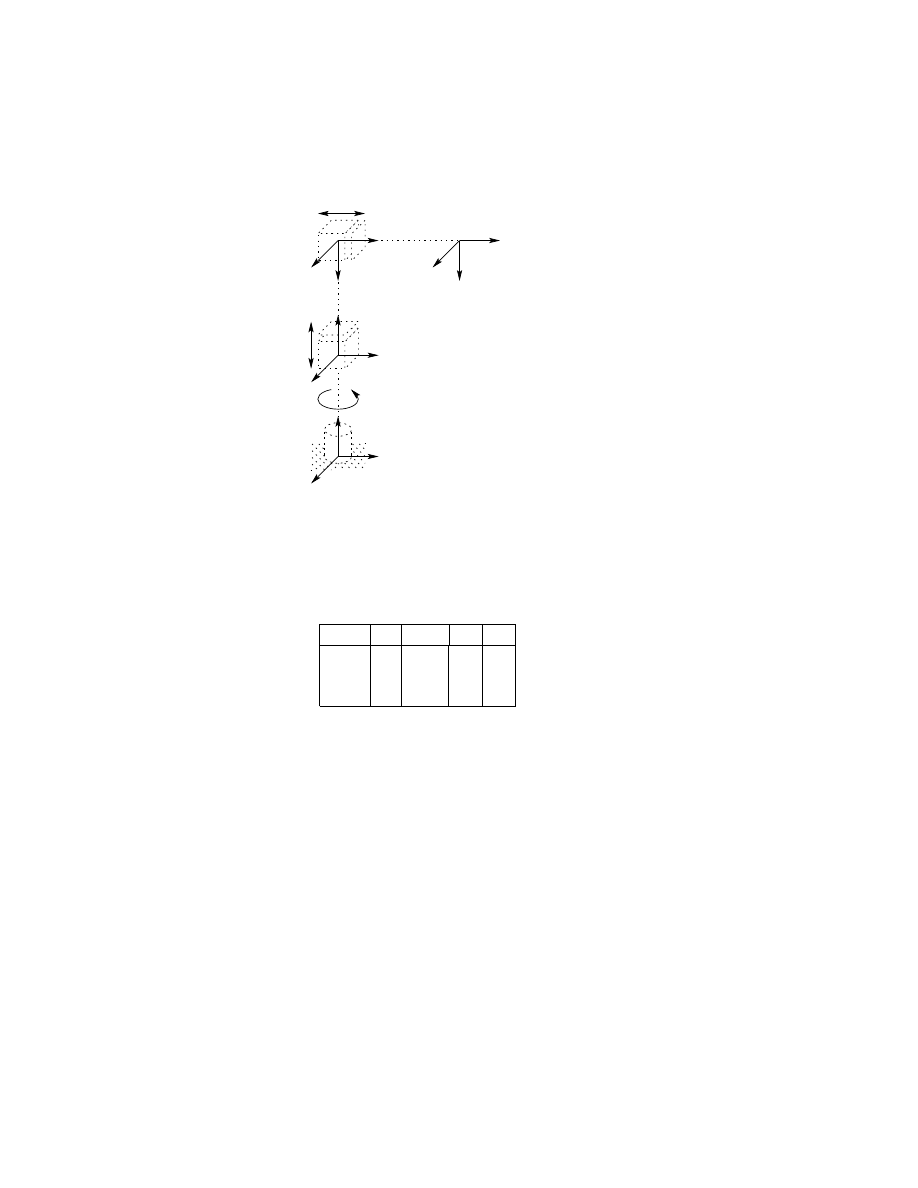
Figure 3.2: Coordinate frames satisfying assumptions DH1 and DH2.
needed from six to four (or even fewer in some cases). In Section 3.2.1 we
will show why, and under what conditions, this can be done, and in Section
3.2.2 we will show exactly how to make the coordinate frame assignments.
3.2.1
Existence and uniqueness issues
Clearly it is not possible to represent any arbitrary homogeneous transforma-
tion using only four parameters. Therefore, we begin by determining just
which homogeneous transformations can be expressed in the form (3.10).
Suppose we are given two frames, denoted by frames 0 and 1, respectively.
Then there exists a unique homogeneous transformation matrix A that takes
the coordinates from frame 1 into those of frame 0. Now suppose the two
frames have two additional features, namely:
(DH1) The axis x
1
is perpendicular to the axis z
0
(DH2) The axis x
1
intersects the axis z
0
as shown in Figure 3.2. Under these conditions, we claim that there exist
unique numbers a, d, θ, α such that
A
= R
z,θ
Trans
z,d
Trans
x,a
R
x,α
.
(3.11)
Of course, since θ and α are angles, we really mean that they are unique to
within a multiple of 2π. To show that the matrix A can be written in this

3.2. DENAVIT HARTENBERG REPRESENTATION
77
form, write A as
A
=
"
R
0
1
O
0
1
0
1
#
(3.12)
and let r
i
denote the i
th
column of the rotation matrix R
0
1
. We will now
examine the implications of the two DH constraints.
If (DH1) is satisfied, then x
1
is perpendicular to z
0
and we have x
1
·z
0
= 0.
Expressing this constraint with respect to o
0
x
0
y
0
z
0
, using the fact that r
1
is
the representation of the unit vector x
1
with respect to frame 0, we obtain
0 = x
0
1
· z
0
0
(3.13)
= [r
11
, r
21
, r
31
]
T
· [0, 0, 1]
T
(3.14)
= r
31
.
(3.15)
Since r
31
= 0, we now need only show that there exist unique angles θ and
α
such that
R
0
1
= R
x,θ
R
x,α
=
c
θ
−s
θ
c
α
s
θ
s
α
s
θ
c
θ
c
α
−c
θ
s
α
0
s
α
c
α
.
(3.16)
The only information we have is that r
31
= 0, but this is enough. First,
since each row and column of R
0
1
must have unit length, r
31
= 0 implies that
r
2
11
+ r
2
21
= 1,
r
2
32
+ r
2
33
= 1
(3.17)
Hence there exist unique θ, α such that
(r
11
, r
21
) = (c
θ
, s
θ
),
(r
33
, r
32
) = (c
α
, s
α
).
(3.18)
Once θ and α are found, it is routine to show that the remaining elements of
R
0
1
must have the form shown in (3.16), using the fact that R
0
1
is a rotation
matrix.
Next, assumption (DH2) means that the displacement between O
0
and
O
1
can be expressed as a linear combination of the vectors z
0
and x
1
. This
can be written as O
1
= O
0
+ dz
0
+ ax
1
. Again, we can express this relation-
ship in the coordinates of o
0
x
0
y
0
z
0
, and we obtain
O
0
1
= O
0
0
+ dz
0
0
+ ax
0
1
(3.19)
78CHAPTER 3. FORWARD KINEMATICS: THE DENAVIT-HARTENBERG CONVENTION
=
0
0
0
+ d
0
0
1
+ a
c
θ
s
θ
0
(3.20)
=
ac
θ
as
θ
d
.
(3.21)
Combining the above results, we obtain (3.10) as claimed. Thus, we see
that four parameters are sufficient to specify any homogeneous transforma-
tion that satisfies the constraints (DH1) and (DH2).
Now that we have established that each homogeneous transformation
matrix satisfying conditions (DH1) and (DH2) above can be represented
in the form (3.10), we can in fact give a physical interpretation to each
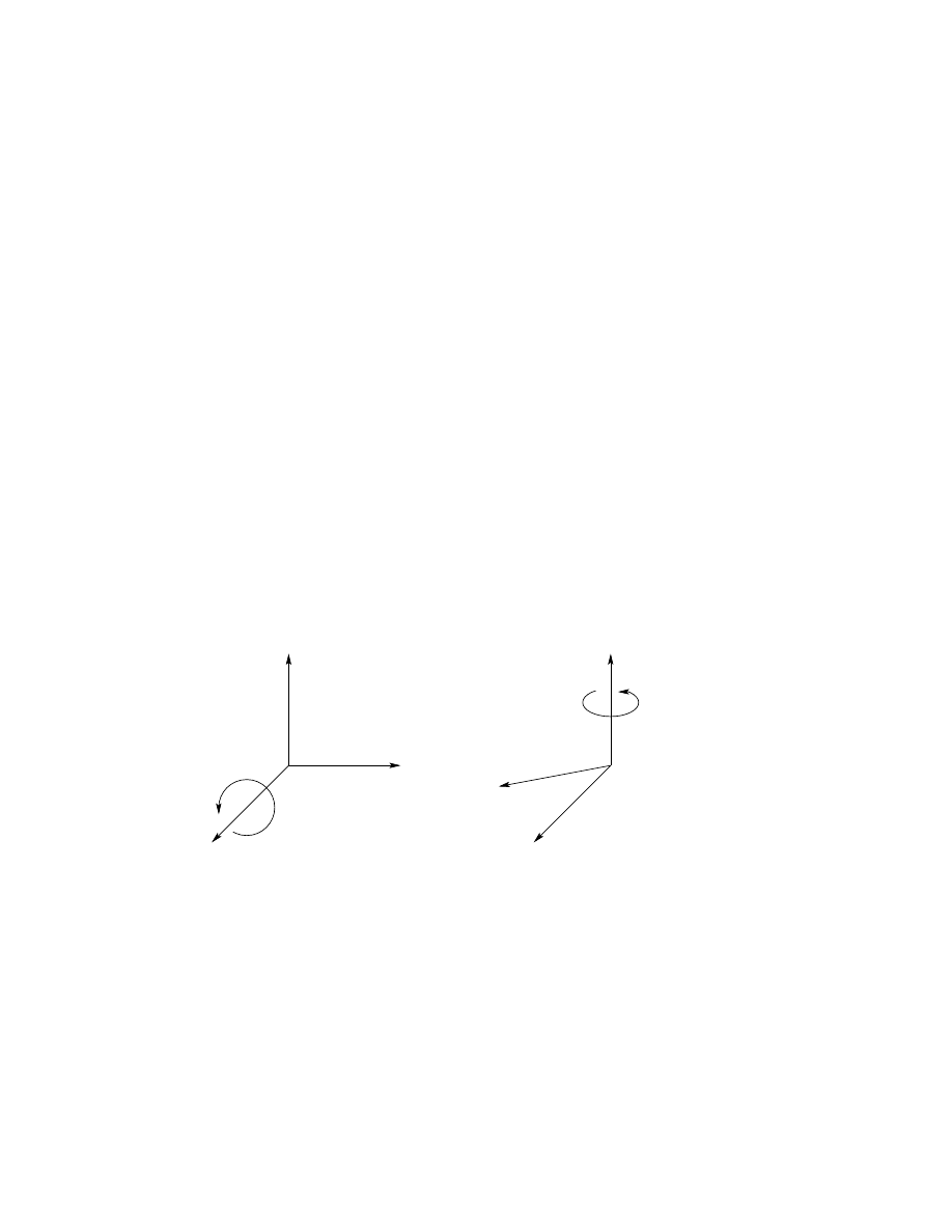
of the four quantities in (3.10). The parameter a is the distance between
the axes z
0
and z
1
, and is measured along the axis x
1
. The angle α is the
angle between the axes z
0
and z
1
, measured in a plane normal to x
1
. The
positive sense for α is determined from z
0
to z
1
by the right-hand rule as
shown in Figure 3.3. The parameter d is the distance between the origin
x
i
α
i
z
i
−1
x
i
θ
i
z
i
−1
x
i
−1
z
i
Figure 3.3: Positive sense for α
i
and θ
i
.
O
0
and the intersection of the x
1
axis with z
0
measured along the z
0
axis.
Finally, θ is the angle between x
0
and x
1
measured in a plane normal to z
0
.
These physical interpretations will prove useful in developing a procedure for
assigning coordinate frames that satisfy the constraints (DH1) and (DH2),
and we now turn our attention to developing such a procedure.

3.2. DENAVIT HARTENBERG REPRESENTATION
79
3.2.2
Assigning the coordinate frames
For a given robot manipulator, one can always choose the frames 0, . . . , n in
such a way that the above two conditions are satisfied. In certain circum-
stances, this will require placing the origin O
i
of frame i in a location that
may not be intuitively satisfying, but typically this will not be the case. In
reading the material below, it is important to keep in mind that the choices
of the various coordinate frames are not unique, even when constrained by
the requirements above. Thus, it is possible that different engineers will
derive differing, but equally correct, coordinate frame assignments for the
links of the robot. It is very important to note, however, that the end re-
sult (i.e., the matrix T
0
n
) will be the same, regardless of the assignment of
intermediate link frames (assuming that the coordinate frames for link n
coincide). We will begin by deriving the general procedure. We will then
discuss various common special cases where it is possible to further simplify
the homogeneous transformation matrix.
To start, note that the choice of z
i
is arbitrary. In particular, from (3.16),
we see that by choosing α
i
and θ
i
appropriately, we can obtain any arbitrary
direction for z
i
. Thus, for our first step, we assign the axes z
0
, . . . , z
n−1
in
an intuitively pleasing fashion. Specifically, we assign z
i
to be the axis of
actuation for joint i + 1. Thus, z
0
is the axis of actuation for joint 1, z
1
is
the axis of actuation for joint 2, etc. There are two cases to consider: (i) if
joint i + 1 is revolute, z
i
is the axis of revolution of joint i + 1; (ii) if joint
i
+ 1 is prismatic, z
i
is the axis of translation of joint i + 1. At first it may
seem a bit confusing to associate z
i
with joint i + 1, but recall that this
satisfies the convention that we established in Section 3.1, namely that joint
i
is fixed with respect to frame i, and that when joint i is actuated, link i
and its attached frame, o
i
x
i
y
i
z
i
, experience a resulting motion.
Once we have established the z-axes for the links, we establish the base
frame. The choice of a base frame is nearly arbitrary. We may choose the
origin O
0
of the base frame to be any point on z
0
. We then choose x
0
, y
0
in
any convenient manner so long as the resulting frame is right-handed. This
sets up frame 0.
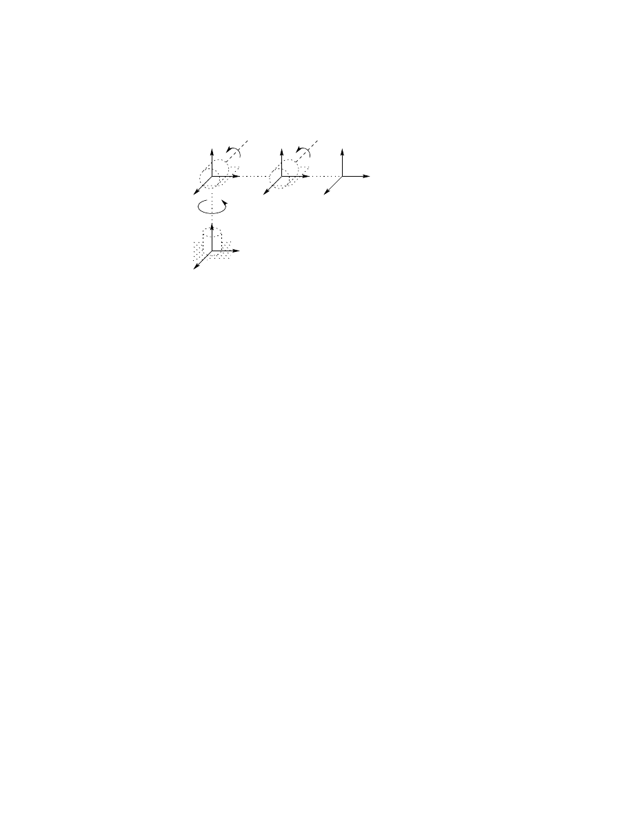
Once frame 0 has been established, we begin an iterative process in which
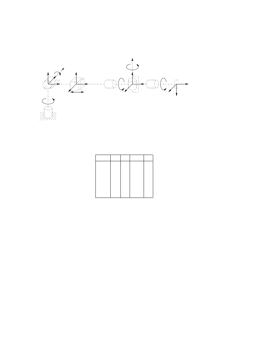
we define frame i using frame i − 1, beginning with frame 1. Figure 3.4 will
be useful for understanding the process that we now describe.
In order to set up frame i it is necessary to consider three cases: (i) the
axes z
i−1
, z
i
are not coplanar, (ii) the axes z
i−1
, z
i
intersect (iii) the axes
z
i−1
, z
i
are parallel. Note that in both cases (ii) and (iii) the axes z
i−1
and
z
i
are coplanar. This situation is in fact quite common, as we will see in

80CHAPTER 3. FORWARD KINEMATICS: THE DENAVIT-HARTENBERG CONVENTION
Figure 3.4: Denavit-Hartenberg frame assignment.
Section 3.3. We now consider each of these three cases.
(i) z
i−1
and z
i
are not coplanar:
If z
i−l
and z
i
are not coplanar, then
there exists a unique line segment perpendicular to both z
i−1
and z
i
such
that it connects both lines and it has minimum length. The line containing
this common normal to z
i−1
and z
i
defines x
i
, and the point where this line
intersects z
i
is the origin O
i
. By construction, both conditions (DH1) and
(DH2) are satisfied and the vector from O
i−1
to O
i
is a linear combination
of z
i−1
and x
i
. The specification of frame i is completed by choosing the
axis y
i
to form a right-hand frame. Since assumptions (DH1) and (DH2) are
satisfied the homogeneous transformation matrix A
i
is of the form (3.10).
(ii) z
i−1
is parallel to z
i
:
If the axes z
i−1
and z
i
are parallel, then there are
infinitely many common normals between them and condition (DH1) does
not specify x
i
completely. In this case we are free to choose the origin O
i
anywhere along z
i
. One often chooses O
i
to simplify the resulting equations.
The axis x
i
is then chosen either to be directed from O
i
toward z
i−1
, along
the common normal, or as the opposite of this vector. A common method
for choosing O
i
is to choose the normal that passes through O
i−1
as the x
i
axis; O
i
is then the point at which this normal intersects z
i
. In this case, d
i
would be equal to zero. Once x
i
is fixed, y
i
is determined, as usual by the
right hand rule. Since the axes z
i−1
and z
i
are parallel, α
i
will be zero in
this case.
(iii) z
i−1
intersects z
i
:
In this case x
i
is chosen normal to the plane
formed by z
i
and z
i−1
. The positive direction of x
i
is arbitrary. The most
3.2. DENAVIT HARTENBERG REPRESENTATION
81
natural choice for the origin O
i
in this case is at the point of intersection of
z
i
and z
i−1
. However, any convenient point along the axis z
i
suffices. Note
that in this case the parameter a
i
equals 0.
This constructive procedure works for frames 0, . . . , n − l in an n-link
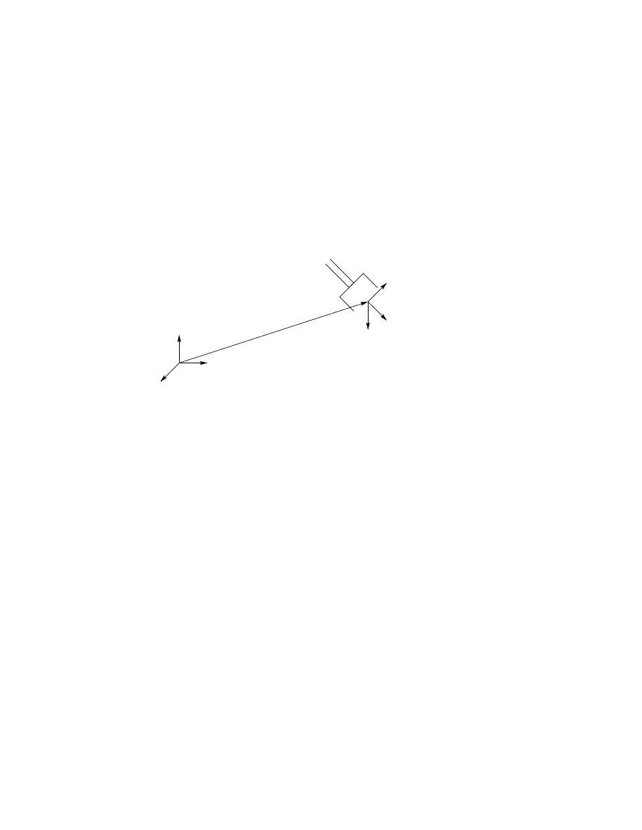
robot. To complete the construction, it is necessary to specify frame n.
The final coordinate system o
n
x
n
y
n
z
n
is commonly referred to as the end-
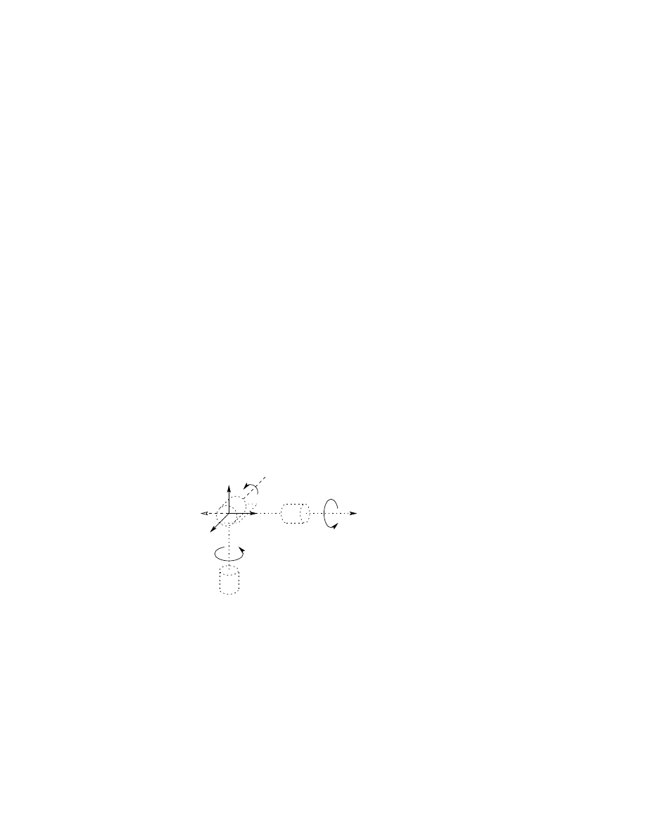
effector or tool frame (see Figure 3.5). The origin O
n
is most often
Note: currently rendering
a 3D gripper...
y
n
≡ s
O
n
O
0
z
0
y
0
x
0
x
n
≡ n
z
n
≡ a
Figure 3.5: Tool frame assignment.
placed symmetrically between the fingers of the gripper. The unit vectors
along the x
n
, y
n
, and z
n
axes are labeled as n, s, and a, respectively. The
terminology arises from fact that the direction a is the approach direction,
in the sense that the gripper typically approaches an object along the a
direction. Similarly the s direction is the sliding direction, the direction
along which the fingers of the gripper slide to open and close, and n is the
direction normal to the plane formed by a and s.
In contemporary robots the final joint motion is a rotation of the end-
effector by θ
n
and the final two joint axes, z
n−1
and z
n
, coincide. In this
case, the transformation between the final two coordinate frames is a trans-
lation along z
n−1
by a distance d
n
followed (or preceded) by a rotation of
θ
n
radians about z
n−1
. This is an important observation that will simplify
the computation of the inverse kinematics in the next chapter.
Finally, note the following important fact. In all cases, whether the joint
in question is revolute or prismatic, the quantities a
i
and α
i
are always
constant for all i and are characteristic of the manipulator. If joint i is pris-
matic, then θ
i
is also a constant, while d
i
is the i
th
joint variable. Similarly,
if joint i is revolute, then d
i
is constant and θ
i
is the i
th
joint variable.

82CHAPTER 3. FORWARD KINEMATICS: THE DENAVIT-HARTENBERG CONVENTION
3.2.3
Summary
We may summarize the above procedure based on the D-H convention in the
following algorithm for deriving the forward kinematics for any manipulator.
Step l: Locate and label the joint axes z
0
, . . . , z
n−1
.
Step 2: Establish the base frame. Set the origin anywhere on the z
0
-axis.
The x
0
and y
0
axes are chosen conveniently to form a right-hand frame.
For i = 1, . . . , n − 1, perform Steps 3 to 5.
Step 3: Locate the origin O
i
where the common normal to z
i
and z
i−1
intersects z
i
. If z
i
intersects z
i−1
locate O
i
at this intersection. If z
i
and z
i−1
are parallel, locate O
i
in any convenient position along z
i
.
Step 4: Establish x
i
along the common normal between z
i−1
and z
i
through
O
i
, or in the direction normal to the z
i−1
− z
i
plane if z
i−1
and z
i
intersect.
Step 5: Establish y
i
to complete a right-hand frame.
Step 6: Establish the end-effector frame o
n
x
n
y
n
z
n
. Assuming the n-th joint
is revolute, set z
n
= a along the direction z
n−1
. Establish the origin
O
n
conveniently along z
n
, preferably at the center of the gripper or at
the tip of any tool that the manipulator may be carrying. Set y
n
= s
in the direction of the gripper closure and set x
n
= n as s × a. If
the tool is not a simple gripper set x
n
and y
n
conveniently to form a
right-hand frame.
Step 7: Create a table of link parameters a
i
, d
i
, α
i
, θ
i
.
a
i
= distance along x
i
from O
i
to the intersection of the x
i
and z
i−1
axes.
d
i
= distance along z
i−1
from O
i−1
to the intersection of the x
i
and
z
i−1
axes. d
i
is variable if joint i is prismatic.
α
i
= the angle between z
i−1
and z
i
measured about x
i
(see Figure
3.3).
θ
i
= the angle between x
i−1
and x
i
measured about z
i−1
(see Figure
3.3). θ
i
is variable if joint i is revolute.
Step 8: Form the homogeneous transformation matrices A
i
by substituting
the above parameters into (3.10).
3.3. EXAMPLES
83
Step 9: Form T
0
n
= A
1
· · · A
n
. This then gives the position and orientation
of the tool frame expressed in base coordinates.
3.3
Examples
In the D-H convention the only variable angle is θ, so we simplify notation
by writing c
i
for cos θ
i
, etc. We also denote θ
1
+ θ
2
by θ
12
, and cos(θ
1
+ θ
2
)
by c
12
, and so on. In the following examples it is important to remember
that the D-H convention, while systematic, still allows considerable freedom
in the choice of some of the manipulator parameters. This is particularly
true in the case of parallel joint axes or when prismatic joints are involved.
Example 3.1 Planar Elbow Manipulator
Consider the two-link planar arm of Figure 3.6. The joint axes z
0
and
y
0
x
0
θ
1
x
1
x
2
θ
2
y
1
y
2
a
1
a
2
Figure 3.6: Two-link planar manipulator. The z-axes all point out of the
page, and are not shown in the figure.
z
1
are normal to the page. We establish the base frame o
0
x
0
y
0
z
0
as shown.
The origin is chosen at the point of intersection of the z
0
axis with the page
and the direction of the x
0
axis is completely arbitrary. Once the base frame
is established, the o
1
x
1
y
1
z
1
frame is fixed as shown by the D-H convention,
where the origin O
1
has been located at the intersection of z
1
and the page.
The final frame o
2
x
2
y
2
z
2
is fixed by choosing the origin O
2
at the end of link 2
as shown. The link parameters are shown in Table 3.1. The A-matrices are

84CHAPTER 3. FORWARD KINEMATICS: THE DENAVIT-HARTENBERG CONVENTION
Table 3.1: Link parameters for 2-link planar manipulator.
Link
a
i
α
i
d
i
θ
i
1
a
1
0
0
θ
∗
1
2
a
2
0
0
θ
∗
2
∗
variable
determined from (3.10) as
A
1
=
c
1
−s
1
0 a
1
c
1
s
1
c
1
0 a
1
s
1
0
0
1
0
0
0
0
1
.
(3.22)
A
2
=
c
2
−s
2
0 a
2
c
2
s
2
c
2
0 a
2
s
2
0
0
1
0
0
0
0
1
(3.23)
The T -matrices are thus given by
T
0
1
= A
1
.
(3.24)
T
0
2
= A
1
A
2
=
c
12
−s
12
0 a
1
c
1
+ a
2
c
12
s
12
c
12
0 a
1
s
1
+ a
2
s
12
0
0
1
0
0
0
0
1
.
(3.25)
Notice that the first two entries of the last column of T
0
2
are the x and y
components of the origin O
2
in the base frame; that is,
x
= a
1
c
1
+ a
2
c
12
(3.26)
y
= a
1
s
1
+ a
2
s
12
are the coordinates of the end-effector in the base frame. The rotational part
of T
0
2
gives the orientation of the frame o
2
x
2
y
2
z
2
relative to the base frame.
⋄
Example 3.2 Three-Link Cylindrical Robot
Consider now the three-link cylindrical robot represented symbolically by
Figure 3.7. We establish O
0
as shown at joint 1. Note that the placement of
3.3. EXAMPLES
85
d
3
d
2
y
3
x
3
z
3
O
3
y
2
y
0
y
1
O
0
O
1
O
2
z
1
z
2
x
2
x
1
x
0
z
0
θ
1
Figure 3.7: Three-link cylindrical manipulator.
Table 3.2: Link parameters for 3-link cylindrical manipulator.
Link
a
i
α
i
d
i
θ
i
1
0
0
d
1
θ
∗
1
2
0
−90
d
∗
2
0
3
0
0
d
∗
3
0
∗
variable
the origin O
0
along z
0
as well as the direction of the x
0
axis are arbitrary.
Our choice of O
0
is the most natural, but O
0
could just as well be placed
at joint 2. The axis x
0
is chosen normal to the page. Next, since z
0
and
z
1
coincide, the origin O
1
is chosen at joint 1 as shown. The x
1
axis is
normal to the page when θ
1
= 0 but, of course its direction will change since
θ
1
is variable. Since z
2
and z
1
intersect, the origin O
2
is placed at this
intersection. The direction of x
2
is chosen parallel to x
1
so that θ
2
is zero.
Finally, the third frame is chosen at the end of link 3 as shown.
The link parameters are now shown in Table 3.2. The corresponding A
86CHAPTER 3. FORWARD KINEMATICS: THE DENAVIT-HARTENBERG CONVENTION
and T matrices are
A
1
=
c
1
−s
1
0
0
s
1
c
1
0
0
0
0
1 d
1
0
0
0
1
(3.27)
A
2
=
1
0
0
0
0
0
1
0
0 −1 0 d
2
0
0
0
1
A
3
=
1 0 0
0
0 1 0
0
0 0 1 d
3
0 0 0
1
T
0
3
= A
1
A
2
A
3
=
c
1
0
−s
1
−s
1
d
3
s
1
0
c
1
c
1
d
3
0
−1
0
d
1
+ d
2
0
0
0
1
.
(3.28)
⋄
Example 3.3 Spherical Wrist
θ
5
θ
4
z
5
x
4
z
4
θ
6
To gripper
x
5
z
3
,
Figure 3.8: The spherical wrist frame assignment.
The spherical wrist configuration is shown in Figure 3.8, in which the
joint axes z
3
, z
4
, z
5
intersect at O. The Denavit-Hartenberg parameters are
shown in Table 3.3. The Stanford manipulator is an example of a manipula-
tor that possesses a wrist of this type. In fact, the following analysis applies
to virtually all spherical wrists.

3.3. EXAMPLES
87
Table 3.3: DH parameters for spherical wrist.
Link
a
i
α
i
d
i
θ
i
4
0
−90
0
θ
∗
4
5
0
90
0
θ
∗
5
6
0
0
d
6
θ
∗
6
∗
variable
We show now that the final three joint variables, θ
4
, θ
5
, θ
6
are the Euler
angles φ, θ, ψ, respectively, with respect to the coordinate frame o
3
x
3
y
3
z
3
. To
see this we need only compute the matrices A
4
, A
5
, and A
6
using Table 3.3
and the expression (3.10). This gives
A
4
=
c
4
0
−s
4
0
s
4
0
c
4
0
0
−1
0
0
0
0
0
1
(3.29)
A
5
=
c
5
0
s
5
0
s
5
0
−c
5
0
0
−1
0
0
0
0
0
1
(3.30)
A
6
=
c
6
−s
6
0
0
s
6
c
6
0
0
0
0
1 d
6
0
0
0
1
.
(3.31)
Multiplying these together yields
T
3
6
= A
4
A
5
A
6
=
"
R
3
6
O
3
6
0
1
#
(3.32)
=
c
4
c
5
c
6
− s
4
s
6
−c
4
c
5
s
6
− s
4
c
6
c
4
s
5
c
4
s
5
d
6
s
4
c
5
c
6
+ c
4
s
6
−s
4
c
5
s
6
+ c
4
c
6
s
4
s
5
s
4
s
5
d
6
−s
5
c
6
s
5
s
6
c
5
c
5
d
6
0
0
0
1
.
Comparing the rotational part R
3
6
of T
3
6
with the Euler angle transforma-
tion (2.51) shows that θ
4
, θ
5
, θ
6
can indeed be identified as the Euler angles
φ
, θ and ψ with respect to the coordinate frame o
3
x
3
y
3
z
3
.
⋄
88CHAPTER 3. FORWARD KINEMATICS: THE DENAVIT-HARTENBERG CONVENTION
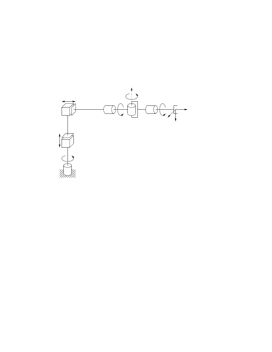
Example 3.4 Cylindrical Manipulator with Spherical Wrist
Suppose that we now attach a spherical wrist to the cylindrical manipula-
tor of Example 3.3.2 as shown in Figure 3.9. Note that the axis of rotation of
d
3
θ
1
d
2
θ
5
θ
4
θ
6
n
s
a
Figure 3.9: Cylindrical robot with spherical wrist.
joint 4 is parallel to z
2
and thus coincides with the axis z
3
of Example 3.3.2.
The implication of this is that we can immediately combine the two previous
expression (3.28) and (3.32) to derive the forward kinematics as
T
0
6
= T
0
3
T
3
6
(3.33)
with T
0
3
given by (3.28) and T
3
6
given by (3.32). Therefore the forward
kinematics of this manipulator is described by
T
0
6
=
c
1
0
−s
1
−s
1
d
1
s
1
0
c
1
c
1
d
3
0
−1
0
d
1
+ d
2
0
0
0
1
c
4
c
5
c
6
− s
4
s
6
−c
4
c
5
s
6
− s
4
c
6
c
4
s
5
c
4
s
5
d
6
s
4
c
5
c
6
+ c
4
s
6
−s
4
c
5
s
6
+ c
4
c
6
s
4
s
5
s
4
s
5
d
6
−s
5
c
6
s
5
c
6
c
5
c
5
d
6
0
0
0
1
(3.34)
=
r
11
r
12
r
13
d
x
r
21
r
22
r
23
d
y
r
31
r
32
r
33
d
z
0
0
0
1

3.3. EXAMPLES
89
where
r
11
= c
1
c
4
c
5
c
6
− c
1
s
4
s
6
+ s
1
s
5
c
6
r
21
= s
1
c
4
c
5
c
6
− s
1
s
4
s
6
− c
1
s
5
c
6
r
31
= −s
4
c
5
c
6
− c
4
s
6
r
12
= −c
1
c
4
c
5
s
6
− c
1
s
4
c
6
− s
1
s
5
c
6
r
22
= −s
1
c
4
c
5
s
6
− s
1
s
4
s
6
+ c
1
s
5
c
6
r
32
= s
4
c
5
c
6
− c
4
c
6
r
13
= c
1
c
4
s
5
− s
1
c
5
r
23
= s
1
c
4
s
5
+ c
1
c
5
r
33
= −s
4
s
5
d
x
= c
1
c
4
s
5
d
6
− s
1
c
5
d
6
− s
1
d
3
d
y
= s
1
c
4
s
5
d
6
+ c
1
c
5
d
6
+ c
1
d
3
d
z
= −s
4
s
5
d
6
+ d
1
+ d
2
.
Notice how most of the complexity of the forward kinematics for this
manipulator results from the orientation of the end-effector while the ex-
pression for the arm position from (3.28) is fairly simple. The spherical
wrist assumption not only simplifies the derivation of the forward kinemat-
ics here, but will also greatly simplify the inverse kinematics problem in the
next chapter.
⋄
Example 3.5 Stanford Manipulator
Consider now the Stanford Manipulator shown in Figure 3.10. This
manipulator is an example of a spherical (RRP) manipulator with a spherical
wrist. This manipulator has an offset in the shoulder joint that slightly
complicates both the forward and inverse kinematics problems.
We first establish the joint coordinate frames using the D-H convention
as shown. The link parameters are shown in the Table 3.4.
It is straightforward to compute the matrices A
i
as
A
1
=
c
1
0 −s
1
0
s
1
0
c
1
0
0 −1
0 0
0
0
0 1
(3.35)
90CHAPTER 3. FORWARD KINEMATICS: THE DENAVIT-HARTENBERG CONVENTION
z
1
θ
2
θ
1
z
0
a
θ
4
d
3
z
2
θ
5
θ
6
n
s
x
0
, x
1
Note: the shoulder (prismatic joint) is mounted wrong.
Figure 3.10: DH coordinate frame assignment for the Stanford manipulator.
Table 3.4: DH parameters for Stanford Manipulator.
Link
d
i
a
i
α
i
θ
i
1
0
0
−90
⋆
2
d
2
0
+90
⋆
3
⋆
0
0
0
4
0
0
−90
⋆
5
0
0
+90
⋆
6
d
6
0
0
⋆
∗
joint variable
A
2
=
c
2
0
s
2
0
s
2
0 −c
2
0
0 1
0 d
2
0 0
0
1
(3.36)
A
3
=
1 0 0
0
0 1 0
0
0 0 1 d
3
0 0 0
1
(3.37)
A
4
=
c
4
0 −s
4
0
s
4
0
c
4
0
0 −1
0 0
0
0
0 1
(3.38)

3.3. EXAMPLES
91
A
5
=
c
5
0
s
5
0
s
5
0 −c
5
0
0 −1
0 0
0
0
0 1
(3.39)
A
6
=
c
6
−s
6
0
0
s
6
c
6
0
0
0
0 1 d
6
0
0 0
1
(3.40)
T
0
6
is then given as
T
0
6
= A
1
· · · A
6
(3.41)
=
r
11
r
12
r
13
d
x
r
21
r
22
r
23
d
y
r
31
r
32
r
33
d
z
0
0
0
1
(3.42)
where
r
11
= c
1
[c
2
(c
4
c
5
c
6
− s
4
s
6
) − s
2
s
5
c
6
] − d
2
(s
4
c
5
c
6
+ c
4
s
6
)
r
21
= s
1
[c
2
(c
4
c
5
c
6
− s
4
s
6
) − s
2
s
5
c
6
] + c
1
(s
4
c
5
c
6
+ c
4
s
6
)
r
31
= −s
2
(c
4
c
5
c
6
− s
4
s
6
) − c
2
s
5
c
6
r
12
= c
1
[−c
2
(c
4
c
5
s
6
+ s
4
c
6
) + s
2
s
5
s
6
] − s
1
(−s
4
c
5
s
6
+ c
4
c
6
)
r
22
= −s
1
[−c
2
(c
4
c
5
s
6
+ s
4
c
6
) + s
2
s
5
s
6
] + c
1
(−s
4
c
5
s
6
+ c
4
c
6
)
r
32
= s
2
(c
4
c
5
s
6
+ s
4
c
6
) + c
2
s
5
s
6
(3.43)
r
13
= c
1
(c
2
c
4
s
5
+ s
2
c
5
) − s
1
s
4
s
5
r
23
= s
1
(c
2
c
4
s
5
+ s
2
c
5
) + c
1
s
4
s
5
r
33
= −s
2
c
4
s
5
+ c
2
c
5
d
x
= c
1
s
2
d
3
− s
1
d
2
+ +d
6
(c
1
c
2
c
4
s
5
+ c
1
c
5
s
2
− s
1
s
4
s
5
)
d
y
= s
1
s
2
d
3
+ c
1
d
2
+ d
6
(c
1
s
4
s
5
+ c
2
c
4
s
1
s
5
+ c
5
s
1
s
2
)
d
z
= c
2
d
3
+ d
6
(c
2
c
5
− c
4
s
2
s
5
).
(3.44)
⋄
Example 3.6 SCARA Manipulator
As another example of the general procedure, consider the SCARA ma-
nipulator of Figure 3.11. This manipulator, which is an abstraction of the
AdeptOne robot of Figure 1.11, consists of an RRP arm and a one degree-
of-freedom wrist, whose motion is a roll about the vertical axis. The first
92CHAPTER 3. FORWARD KINEMATICS: THE DENAVIT-HARTENBERG CONVENTION
z
0
z
1
d
3
θ
4
x
2
y
2
x
0
y
0
θ
1
θ
2
x
1
y
1
y
3
y
4
x
3
x
4
z
2
z
3
,
z
4
Figure 3.11: DH coordinate frame assignment for the SCARA manipulator.
Table 3.5: Joint parameters for SCARA.
Link
a
i
α
i
d
i
θ
i
1
a
1
0
0
⋆
2
a
2
180
0
⋆
3
0
0
⋆
0
4
0
0
d
4
⋆
∗
joint variable
step is to locate and label the joint axes as shown. Since all joint axes are
parallel we have some freedom in the placement of the origins. The origins
are placed as shown for convenience. We establish the x
0
axis in the plane
of the page as shown. This is completely arbitrary and only affects the zero
configuration of the manipulator, that is, the position of the manipulator
when θ
1
= 0.
The joint parameters are given in Table 3.5, and the A-matrices are as

3.3. EXAMPLES
93
follows.
A
1
=
c
1
−s
1
0 a
1
c
1
s
1
c
1
0 a
1
s
1
0
0
1
0
0
0
0
1
(3.45)
A
2
=
c
2
s
2
0
a
2
c
2
s
2
−c
2
0
a
2
s
2
0
0
−1
0
0
0
0
1
(3.46)
A
3
=
1 0 0
0
0 1 0
0
0 0 1 d
3
0 0 0
1
(3.47)
A
4
=
c
4
−s
4
0
0
s
4
c
4
0
0
0
0
1 d
4
0
0
0
1
.
(3.48)
The forward kinematic equations are therefore given by
T
0
4
= A
1
· · · A
4
=
c
12
c
4
+ s
12
s
4
−c
12
s
4
+ s
12
c
4
0
a
1
c
1
+ a
2
c
12
s
12
c
4
− c
12
s
4
−s
12
s
4
− c
12
c
4
0
a
1
s
1
+ a
2
s
12
0
0
−1
−d
3
− d
4
0
0
0
1
.
(3.49)
⋄
94CHAPTER 3. FORWARD KINEMATICS: THE DENAVIT-HARTENBERG CONVENTION
3.4
Problems
1. Verify the statement after Equation (3.18) that the rotation matrix R
has the form (3.16) provided assumptions DH1 and DH2 are satisfied.
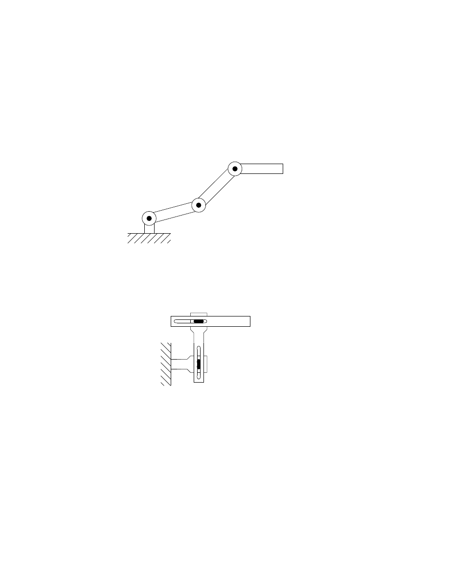
2. Consider the three-link planar manipulator shown in Figure 3.12. Derive
Figure 3.12: Three-link planar arm of Problem 3-2.
the forward kinematic equations using the DH-convention.
3. Consider the two-link cartesian manipulator of Figure 3.13. Derive
Figure 3.13: Two-link cartesian robot of Problem 3-3.
the forward kinematic equations using the DH-convention.
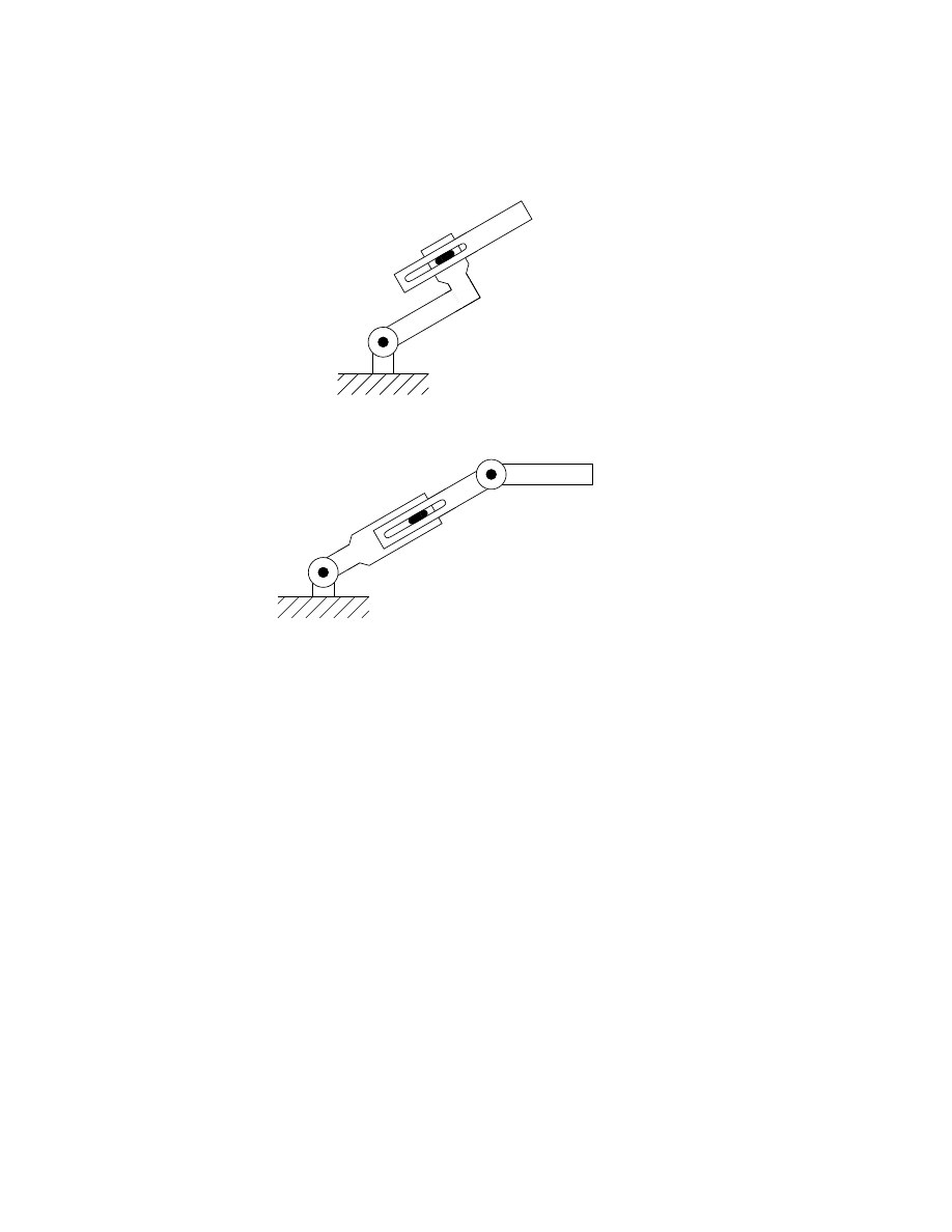
4. Consider the two-link manipulator of Figure 3.14 which has joint 1
revolute and joint 2 prismatic. Derive the forward kinematic equations
using the DH-convention.
5. Consider the three-link planar manipulator of Figure 3.15 Derive the
forward kinematic equations using the DH-convention.
3.4. PROBLEMS
95
Figure 3.14: Two-link planar arm of Problem 3-4.
Figure 3.15: Three-link planar arm with prismatic joint of Problem 3-5.
6. Consider the three-link articulated robot of Figure 3.16. Derive the
forward kinematic equations using the DH-convention.
7. Consider the three-link cartesian manipulator of Figure 3.17. Derive
the forward kinematic equations using the DH-convention.
8. Attach a spherical wrist to the three-link articulated manipulator of
Problem 3-6 as shown in Figure 3.18. Derive the forward kinematic
equations for this manipulator.
9. Attach a spherical wrist to the three-link cartesian manipulator of
Problem 3-7 as shown in Figure 3.19. Derive the forward kinematic
equations for this manipulator.
10. Consider the PUMA 260 manipulator shown in Figure 3.20. Derive
the complete set of forward kinematic equations, by establishing appro-
priate D-H coordinate frames, constructing a table of link parameters,
forming the A-matrices, etc.
96CHAPTER 3. FORWARD KINEMATICS: THE DENAVIT-HARTENBERG CONVENTION
Figure 3.16: Three-link articulated robot.
Figure 3.17: Three-link cartesian robot.
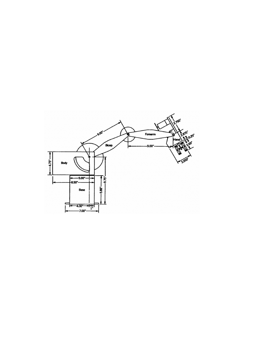
11. Repeat Problem 3-9 for the five degree-of-freedom Rhino XR-3 robot
shown in Figure 3.21. (Note: you should replace the Rhino wrist with
the sperical wrist.)
12. Suppose that a Rhino XR-3 is bolted to a table upon which a coordi-
nate frame o
s
x
s
y
s
z
s
is established as shown in Figure 3.22. (The frame
o
s
x
s
y
x
z
s
is often referred to as the station frame.) Given the base
frame that you established in Problem 3-11, find the homogeneous
transformation T
s
0
relating the base frame to the station frame. Find
the homogeneous transformation T
s
5
relating the end-effector frame to
the station frame. What is the position and orientation of the end-
effector in the station frame when θ
1
= θ
2
= · · · = θ
5
= 0?
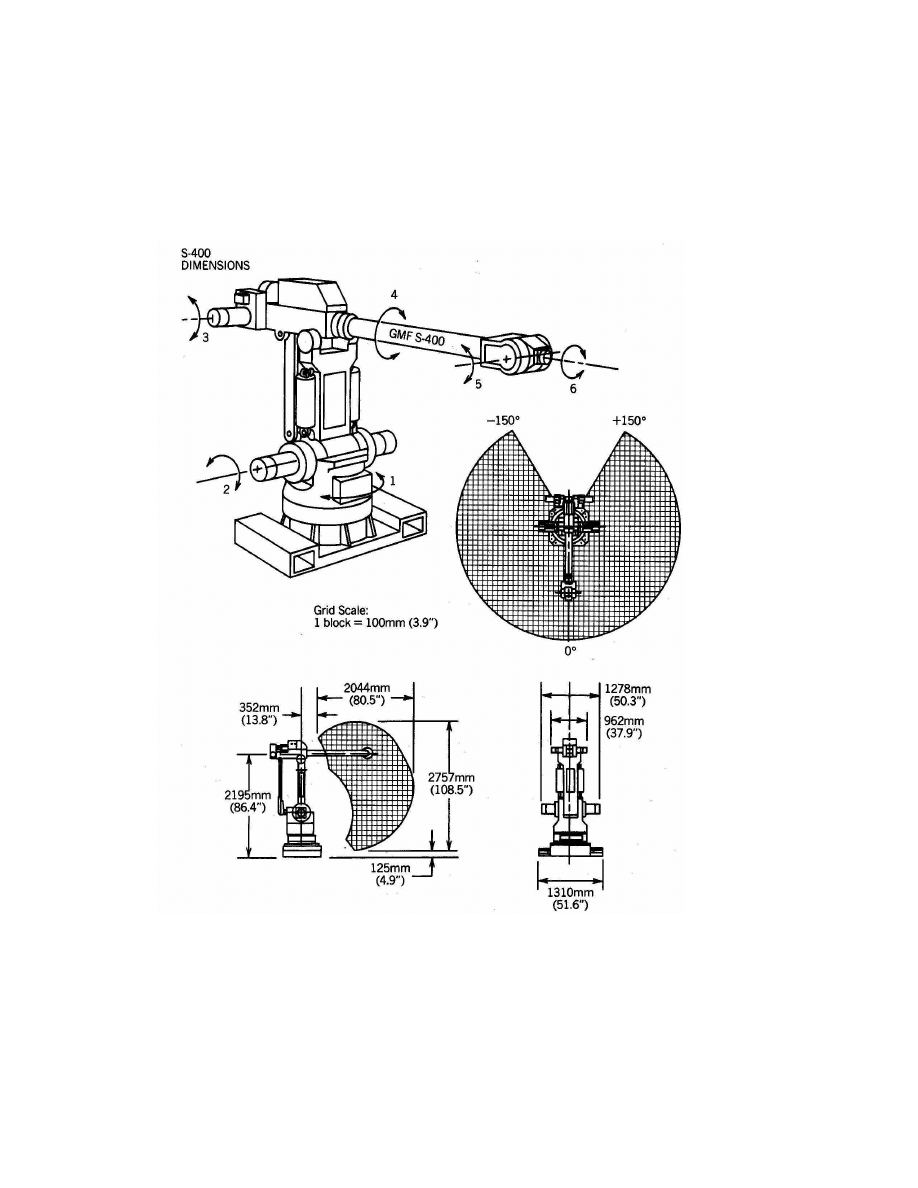
13. Consider the GMF S-400 robot shown in Figure 3.23 Draw the sym-
bolic representation for this manipulator. Establish DH-coordinate
frames and write the forward kinematic equations.
3.4. PROBLEMS
97
Figure 3.18: Elbow manipulator with spherical wrist.
Figure 3.19: Cartesian manipulator with spherical wrist.
98CHAPTER 3. FORWARD KINEMATICS: THE DENAVIT-HARTENBERG CONVENTION
Figure 3.20: PUMA 260 manipulator.
3.4. PROBLEMS
99
Figure 3.21: Rhino XR-3 robot.
100CHAPTER 3. FORWARD KINEMATICS: THE DENAVIT-HARTENBERG CONVENTION
Figure 3.22: Rhino robot attached to a table. From: A Robot Engineering
Textbook
, by Mohsen Shahinpoor. Copyright 1987, Harper & Row Publish-
ers, Inc
3.4. PROBLEMS
101
Figure 3.23: GMF S-400 robot. (Courtesy GMF Robotics.)

102CHAPTER 3. FORWARD KINEMATICS: THE DENAVIT-HARTENBERG CONVENTION
Wyszukiwarka
Podobne podstrony:
Wykł 1B wstępny i kinematyka
Wyklad 06 kinematyka MS
Wyklad 05 kinematyka MS
3 Rodzaje jednorodnych transformacji stosowanych w kinematy
04 Analiza kinematyczna manipulatorów robotów metodą macierz
Mechanika Techniczna I Skrypt 2 4 Kinematyka
03 Kinematyka
fizyka 2 KINEMATYKA PUNKTU MATERIALNEGO
kinematyka manipulatora
kinematyka
zestaw 3 kinematyka
03 Kinematykaid 4394 Nieznany
L6 Kinematyka 2
Kinematyka ukladu korbowego
więcej podobnych podstron