ABUTMENTS

• The Structure upon which the ends of a Bridge

rests is referred to as an

Abutment

• The most common type of Abutment Structure

is a Retaining Wall, Although other types of
Abutments are also possible and are used

• A retaining wall is used to hold back an earth

embankment or water and to maintain a
sudden change in elevation.

• Abutment serves following functions

o Distributes the loads from Bridge Ends to

the ground

o Withstands any loads that are directly

imposed on it

o Provides vehicular and pedestrian access

to the bridge

• In case of Retaining wall type Abutment

bearing capacity and sliding resistance of the
foundation materials and overturning stability
must be checked

TYPES OF ABUTMENTS

• Sixteenth edition of the AASHTO (1996) standard

specification classifies abutments into four types:

o Stub abutments,
o partial-depth abutments,
o full-depth abutments; and
o Integral abutments.

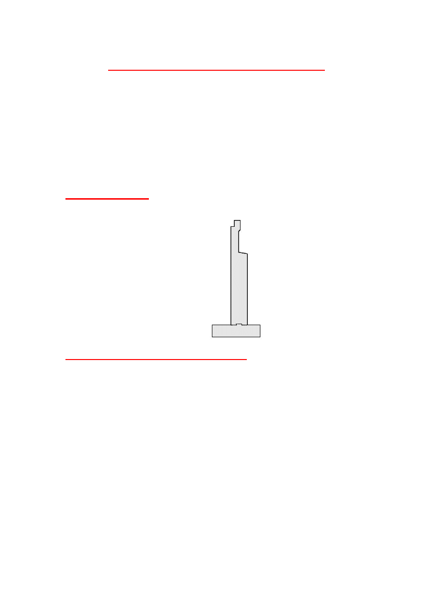
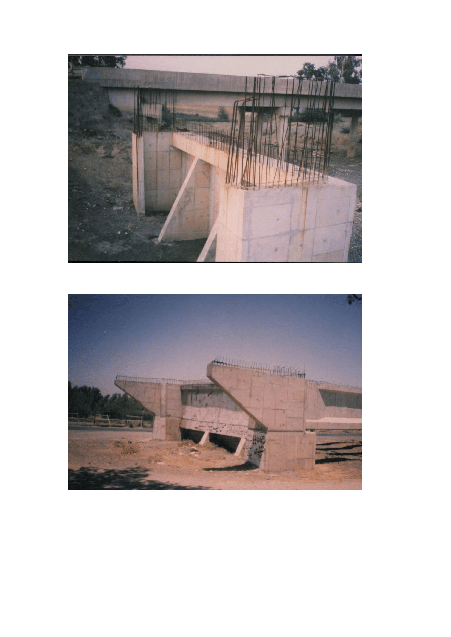
Stub Abutment

Partial-Depth

Abutment

Partial Depth abutments are located
approximately at mid-depth of the front slope
of the approach embankment. The higher
backwall and wingwalls may retain fill
material, or the embankment slope may
continue hehind the backwall. In the latter
case, a structural approach slab or end span
desing must bridge the space over the fill slope
and curtain walls are provided to close off the
open area

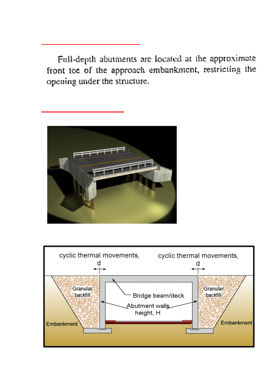
Full-Depth

Abutment

Integral

Abutment

Peck, Hanson Thornburn Classification

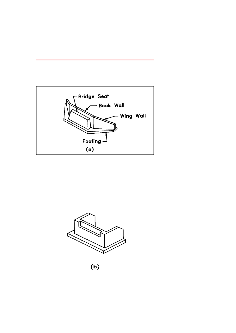
A gravity abutment with wing walls is an abutment that consists of a
bridge seat, wing walls, back wall, and footing.

A U-abutment is an abutment whose, wing walls are perpendicular to
the bridge seat

Gravity Abutment with Wing Walls

U Abutment

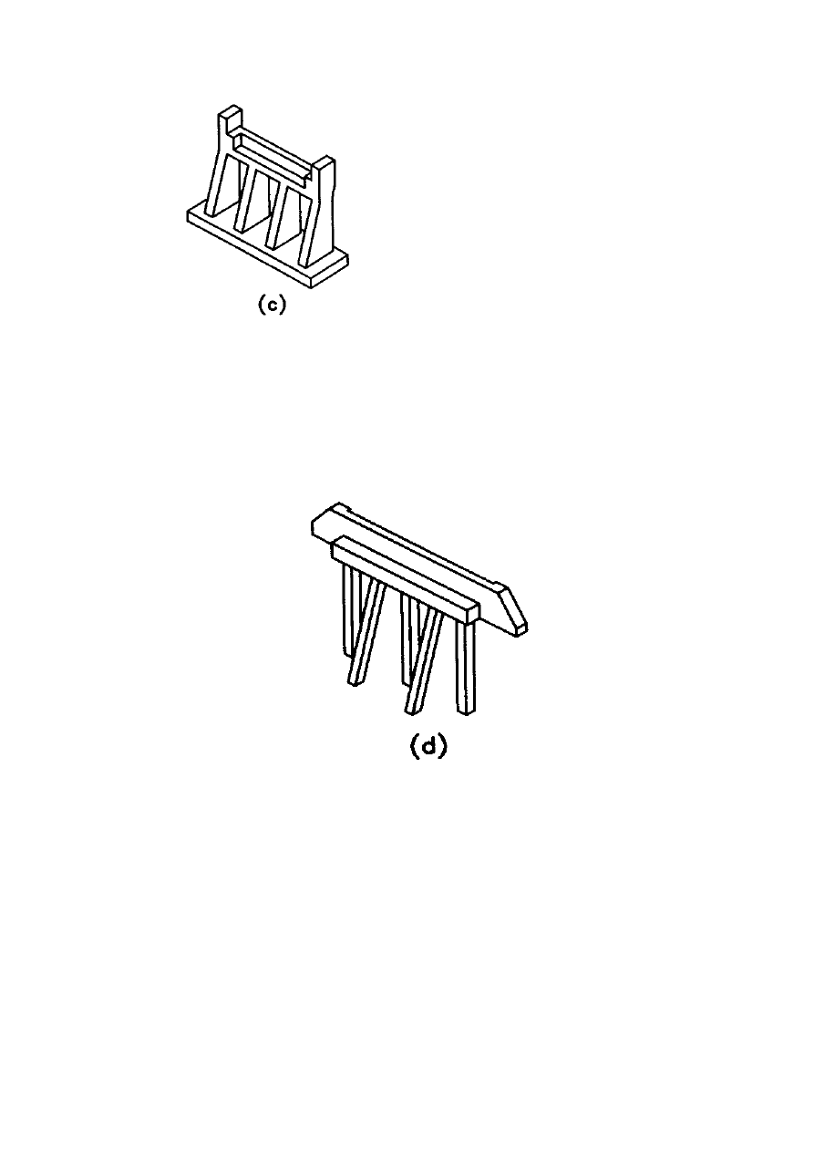
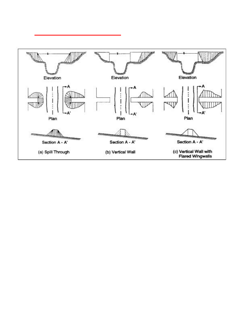
Spill-through abutment consists of a beam that supports the bridge seat, two
or more columns supporting the beam, and a footing supporting the columns.
The columns are embedded up to the bottom of the beam in the fill, which
extends on its natural slope in front of

the abutment.

Pile-bent abutments. A pile-bent abutment with stub wings is
another type of spill-through abutment, where a row of driven piles

supports the beam.

Pile Bent Abutment

Spill Through Abutment

Other Types of Abutments

SELECTION OF ABUTMENTS:

The procedure of selecting the most appropriate type
of abutments can be based on the following
consideration:

1. Construction and maintenance cost

2. Cut or fill earthwork situation

3. Traffic maintenance during construction

4. Construction period

5. Safety of construction workers

6. Availability and cost of backfill material

7. Superstructure depth

8. Size of abutment

9. Horizontal and vertical alignment changes

10. Area of excavation

11. Aesthetics and similarity to adjacent

structures

12. Previous experience with the type of

abutment

13. Ease of access for inspection and

maintenance.

14. Anticipated life, loading condition, and

acceptability of deformations.

LIMIT STATES

When abutments fail to satisfy their intended

design function, they are considered to reach “limit

states.” Limit states can be categorized into two

types:

1) ULTIMATE LIMIT STATES.

An abutment reaches an ultimate limit state when:

i.)

The strength of a least one of its

components is fully mobilized or

ii.)

The structure becomes unstable.

In the ultimate limit state an abutment may experience
serious distress and structural damage, both local and
global. In addition, various failure modes in the soil that
supports the abutment can also be identified. These are
also called ultimate limit states, they include bearing
capacity failure, sliding, overturning, and overall instability.

2) SERVICEABILITY LIMIT STATES.

An abutment experiences a serviceability limit state when
it fails to perform its intended design function fully, due to
excessive deformation or deterioration. Serviceability limit
states include excessive total or differential settlement,
lateral movement, fatigue, vibration, and cracking.

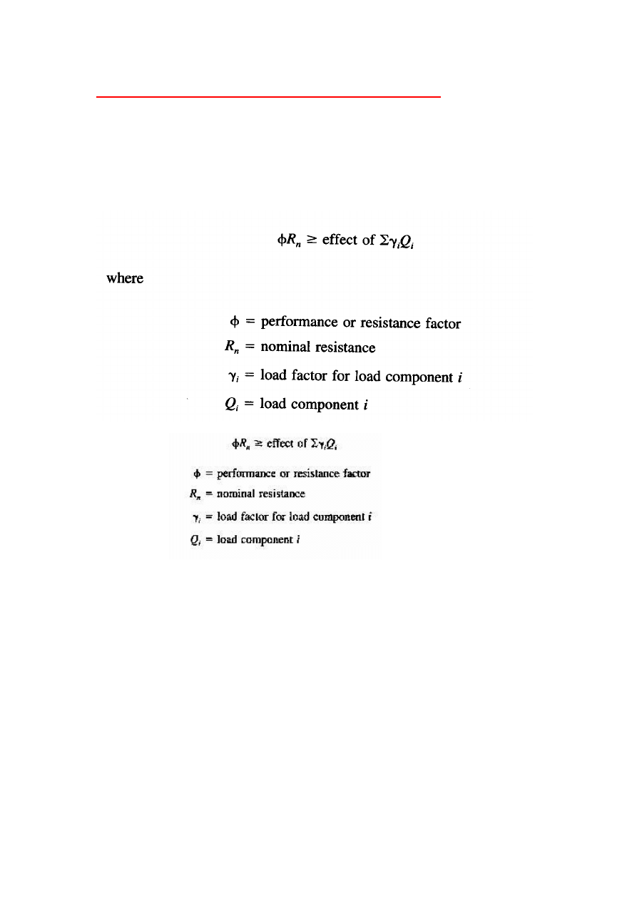
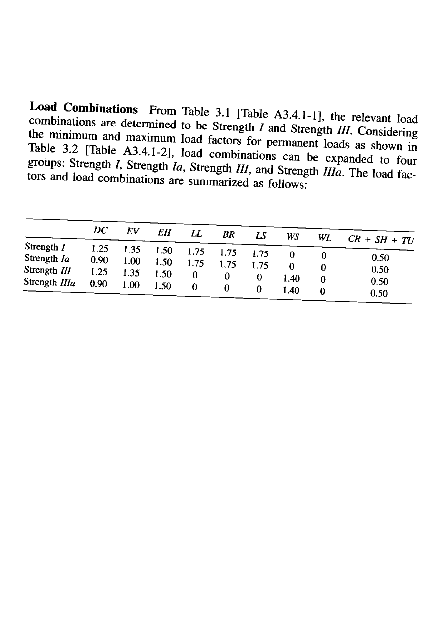
LOAD AND PERFORMANCE FACTORS

The AASHTO (1990) bridge specifications require the

use of the load and resistance factor design (LRFD)
method in the substructure design. A mathematical
statement of LRFD can be expressed as

i) Load Factors :

Load factors are applied to loads to account for
uncertainties in selecting loads and load effects. The load
factors used in the first edition of the AASHTO (1994)
LRFD bridge specifications are shown in Tables 3.1 and
3.2. of the Text.

ii) Performance Factors:

Performance or resistance factors are used to account for
uncertainties in structural properties, soil properties,
variability in workmanship, and inaccuracies in the design
equations used to estimate the capacity. These factors are

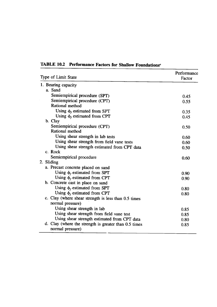
used for design ate the ultimate limit state suggested
values of performance factors for shallow foundations are
listed in

table 10.2

FORCES ON ABUTMENTS

Earth pressures exerted on an abutment can be

classified according to the direction and the
magnitude of the abutment movement.

1) At-rest Earth Pressure

When the wall is fixed rigidly and does not move,
the pressure exerted by the soil on the wall is called
at-rest earth pressure.

2) Active Earth Pressure

:

When a wall moves away from the backfill, the earth
pressure decreases (active pressure)

3) Passive Earth Pressure

When it moves toward the backfill, the earth

pressure increases (passive pressure).

Table 10.3

, obtained through experimental data and

finite element analyses (Clough and Duncan, 1991),
gives approximate magnitudes of wall movements
required to reach minimum active and maximum
passive earth pressure conditions. Observation

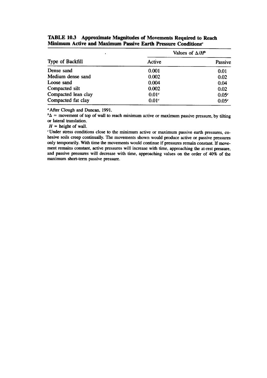
1. The required movements for the extreme conditions are

approximately proportional to the wall height.

2. The movement required to reach the maximum passive pressure

is about 10 times as great as that required to reach the minimum

active pressure for walls of the same height.

3. The movement required to reach the extreme conditions for

dense and incompressible soils is smaller than those for loose

and compressible soil.

For any cohesionless backfill, conservative and simple

guidelines for the maximum movements required to reach the
extreme cases are provided by Clough and Duncan (1991).

For minimum active pressure, the movements no more than about 1 mm

in 240 mm (

∆

/H = 0.004) and for maximum passive pressure about 1 mm

in 24 mm (

∆

/H = 0.004).

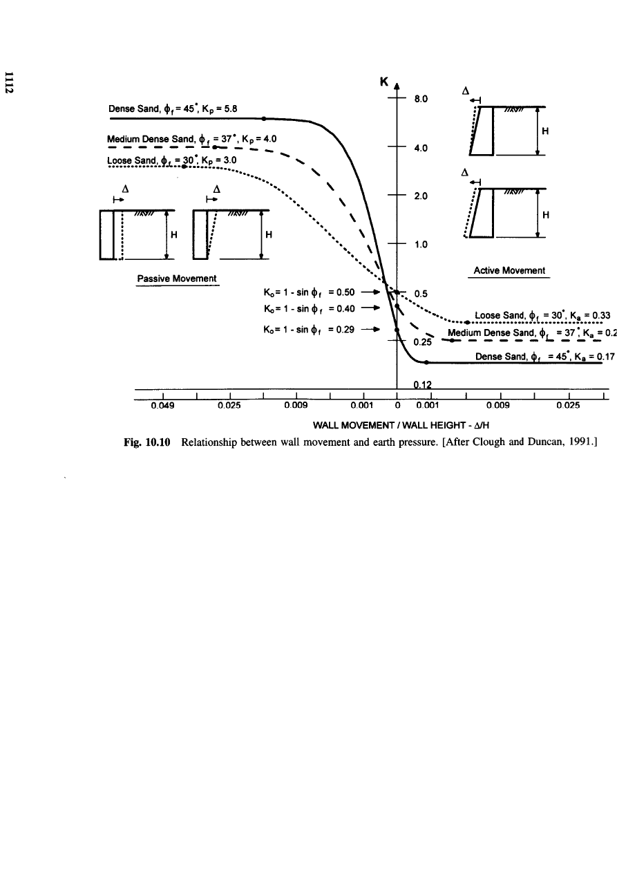
As shown in

figure 10.10:

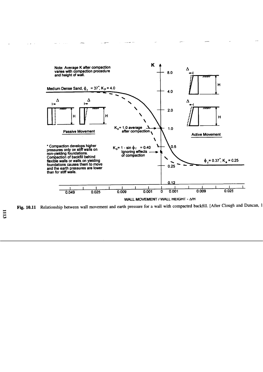
The value for the earth pressure coefficient varies with

wall displacement and eventually remains constant after

sufficiently large displacements.

The change of pressures also varies with the type of soil,

that is, the pressures in the dense sand change more
quickly with wall movement.

METHODS FOR ESTIMATING K

A

AND K

P

Coulomb

in 1776 and

Rankine

in 1856 developed simple methods for

calculating the active and passive earth pressures exerted on

retaining structures. Caquot and Kerisel (1948) developed the
more generally applicable

log spiral theory

, where the movements of

walls are sufficiently large so that the shear strength of the backfill

soil is fully mobilized, and where the strength properties of the
backfill can be estimated with sufficient accuracy, these methods

of calculation are useful for practical purposes.

Coulomb’s trial wedge method can be used for irregular backfill

configurations and Rankine’s theory and the log spiral analysis can

be used for more regular configurations. Each of these methods
will be discussed below.

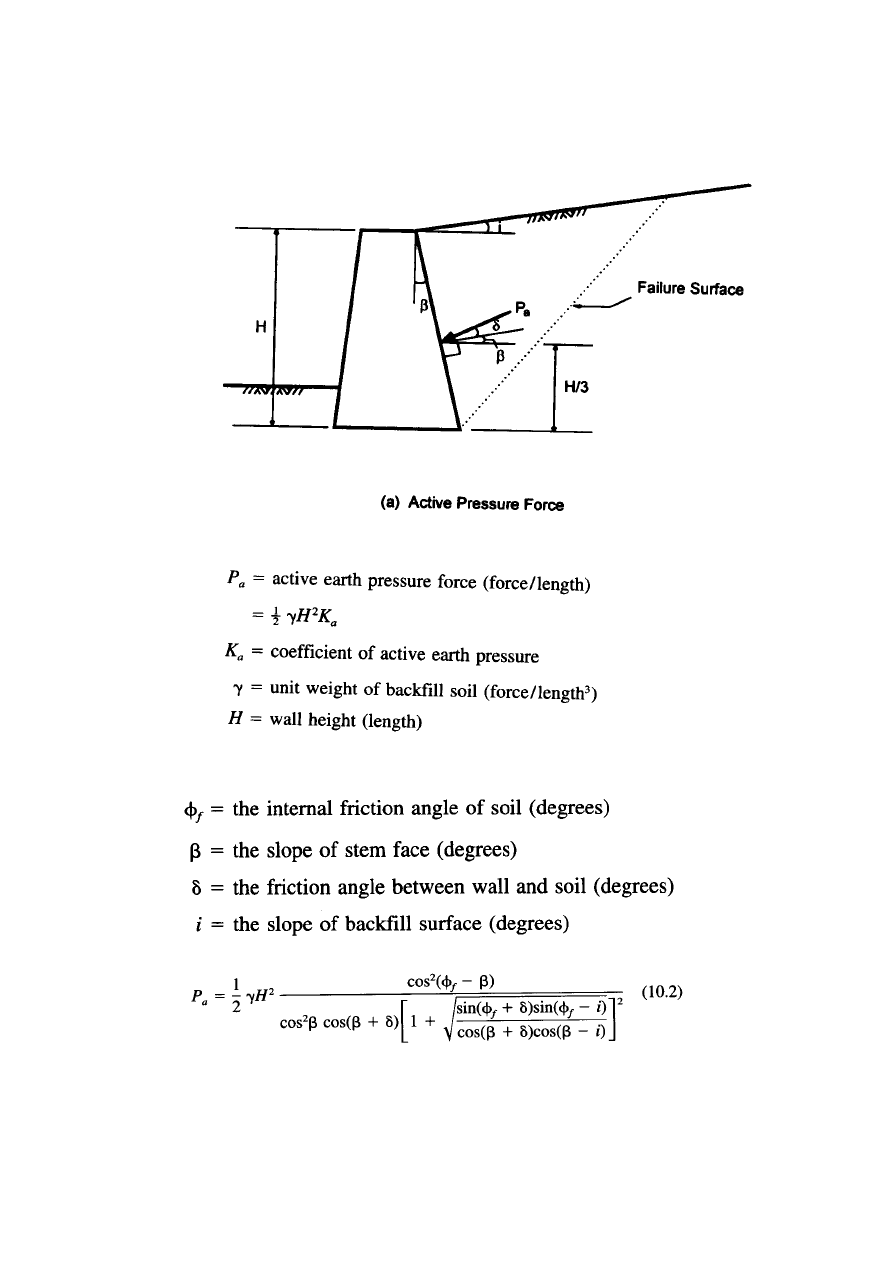
COULOMB THEORY:

The coulomb theory, the first rational solution to the earth

pressure problem, is based on the concept that the lateral force

exerted on a wall by the backfill can be evaluated by analysis of the
equilibrium of a wedge-shaped mass of soil bounded by the back of

the wall, the backfill surface, and a surface of sliding through the
soil. The assumptions in this analysis are
1. The surface of sliding through the soil is a straight line.

2. The full strength of the soil is mobilized to resist sliding (shear

failure) through the soil.

i)

Active Pressure

: A graphical illustration for the mechanism for

active failure according to the coulomb theory is shown in

Figure 10.12a

.

The active earth pressure force can be

expressed as:

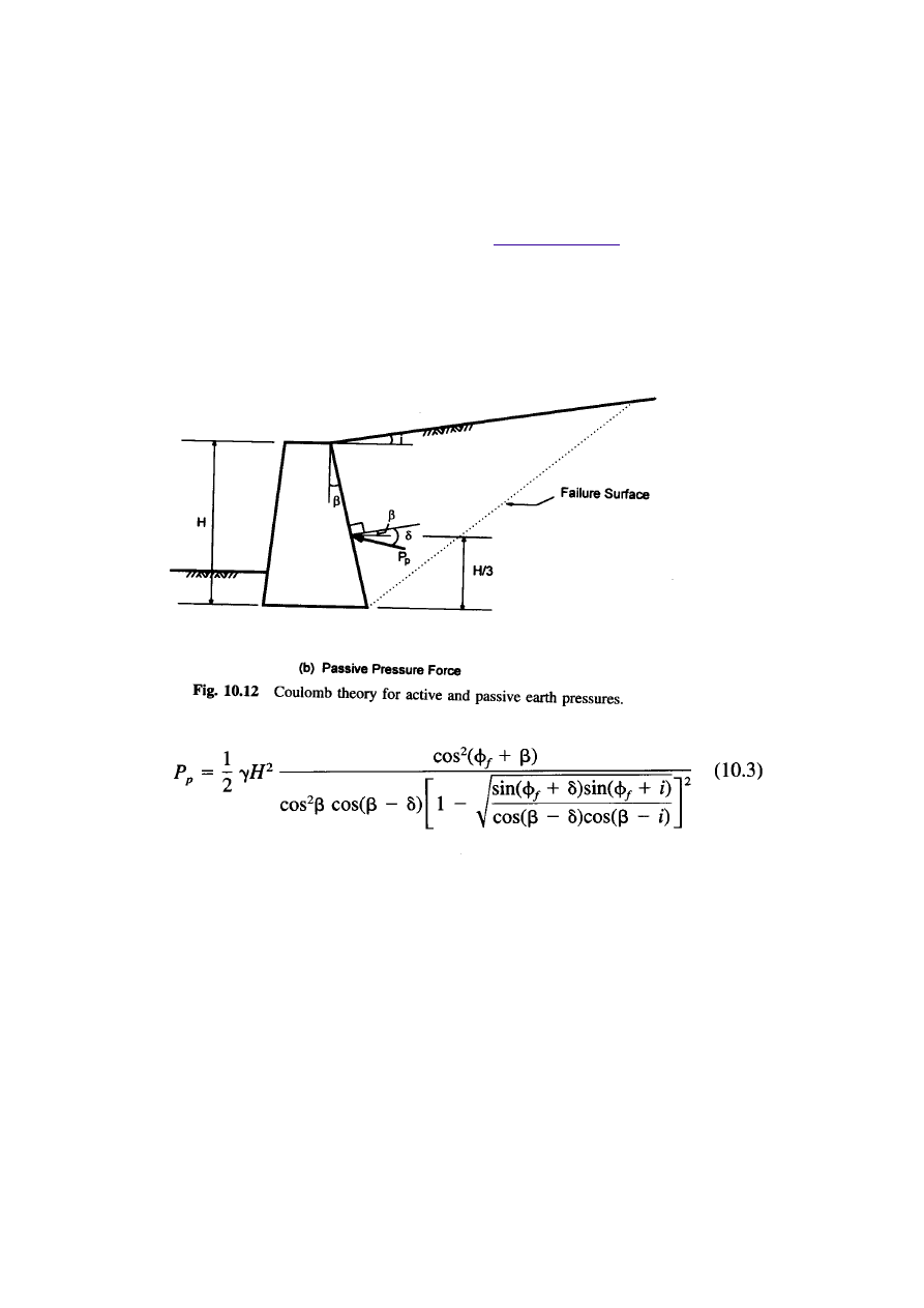
Passive Pressure

:

The coulomb theory can be used to evaluate passive resistance,
using the same basic assumptions.

Figure 10.12b

shows the failure

mechanism for the passive case. The passive earth pressure force,
Pp. can be expressed as follows:

The basic assumption in the coulomb theory is that

the surface of

sliding is a plane

. This assumption does not affect appreciably the

accuracy for the active case. However, for the passive case, values of

p

p

calculated by the coulomb theory can be much larger than can

actually be mobilized, especially when the value of δ exceeds about

one half of ϕ

f .

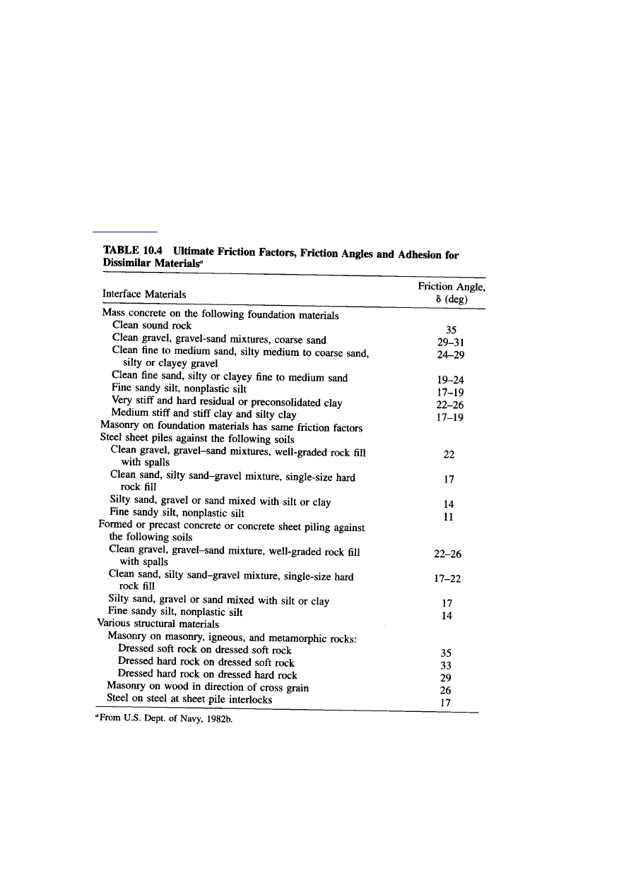
Wall Friction:friction between the wall and backfill has an important
effect on the magnitude of earth pressures and an even more

important effect on the direction of the earth pressure force .

Table 10.4

presents values of the maximum possible wall friction

angle for various wall materials and soil types.

RANKINE THEORY:

The Rankine theory is applicable to conditions

where the wall friction angle

(

ϕ) is equal to the slope of the backfill

surface (I). As in the case of the coulomb theory, it is assumed that the

strength of the soil is fully mobilized.

Table 10.4

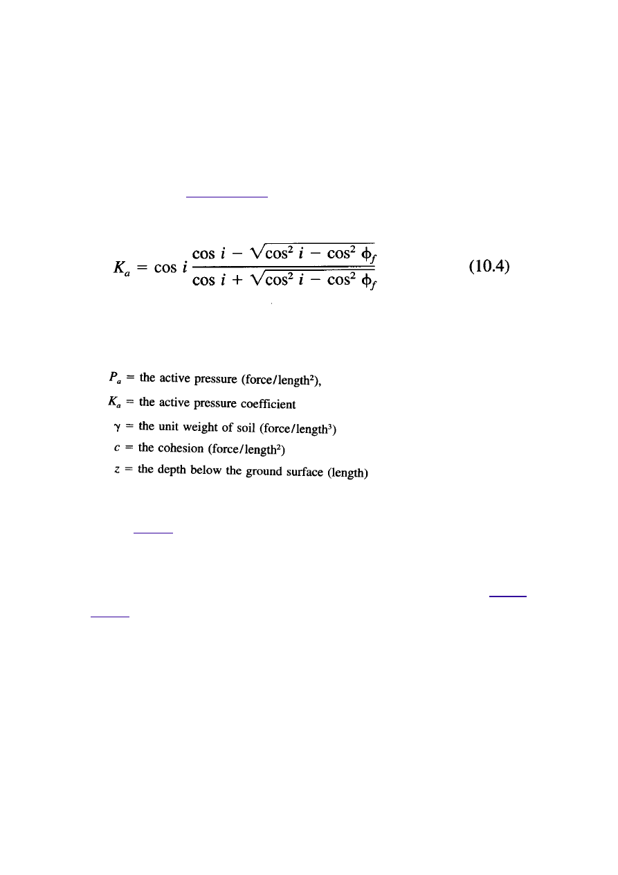
i) Active Pressure:

The active earth pressure considered in the Rankine theory is

illustrated in

Figure 10.13

a for a level backfill condition. The

coefficient of active earth pressure, k

a,

can be expressed as:

When the ground surface is horizontal, that is, when I =0, k

a

can be

expressed as

The variation of active pressure with depth is linear, as shown in

figure

10.13b

. If the backfill is cohesive, the soil is theoretically in a

tension zone down to a depth of 2c/γ(k

a

)

2

. However, a tension crack is

likely to develop in that zone and may be filled with water, so that

hydrostatic pressure will be exerted on the wall, as shown in

figure

10.13c

.

ii) Passive Pressure:

The Rankine theory can also be applied to passive

pressure conditions. The pasive earth pressure coefficient (kp) can be

expressed as

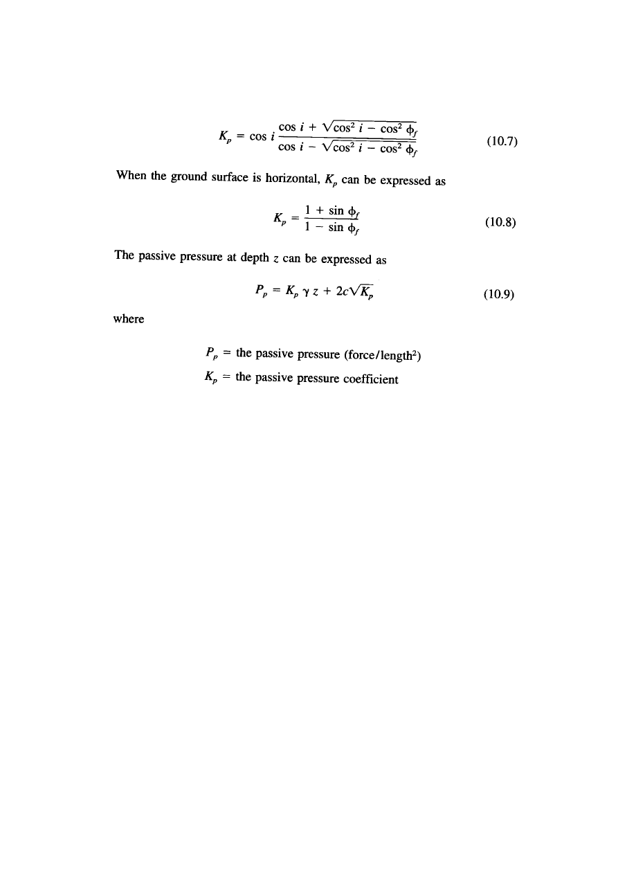
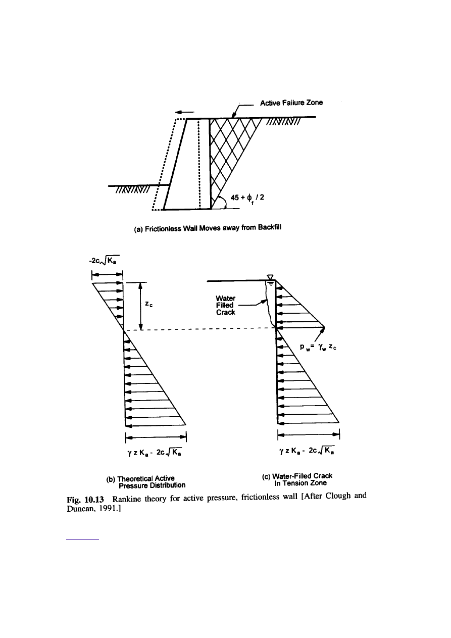
Fig10.13

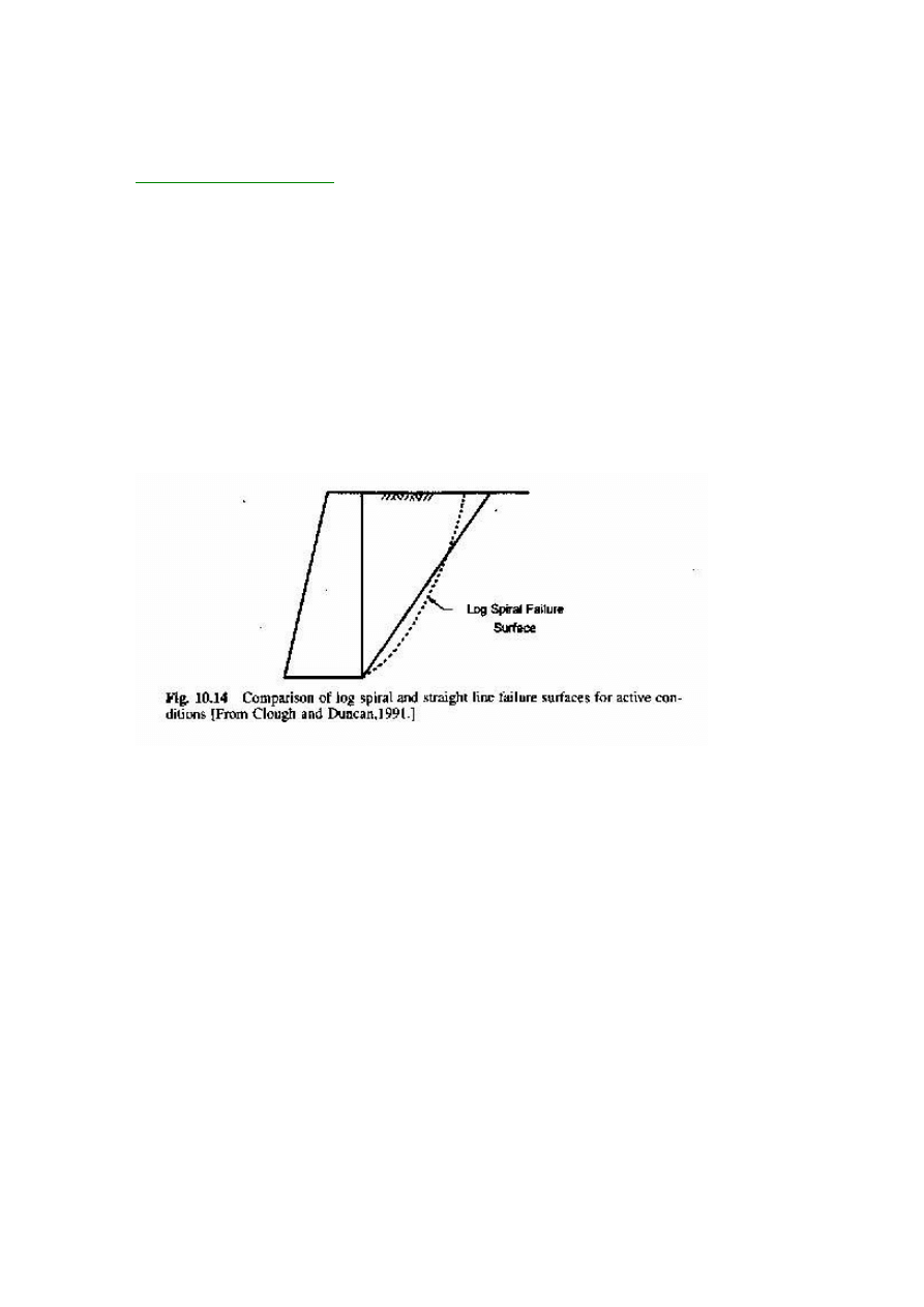
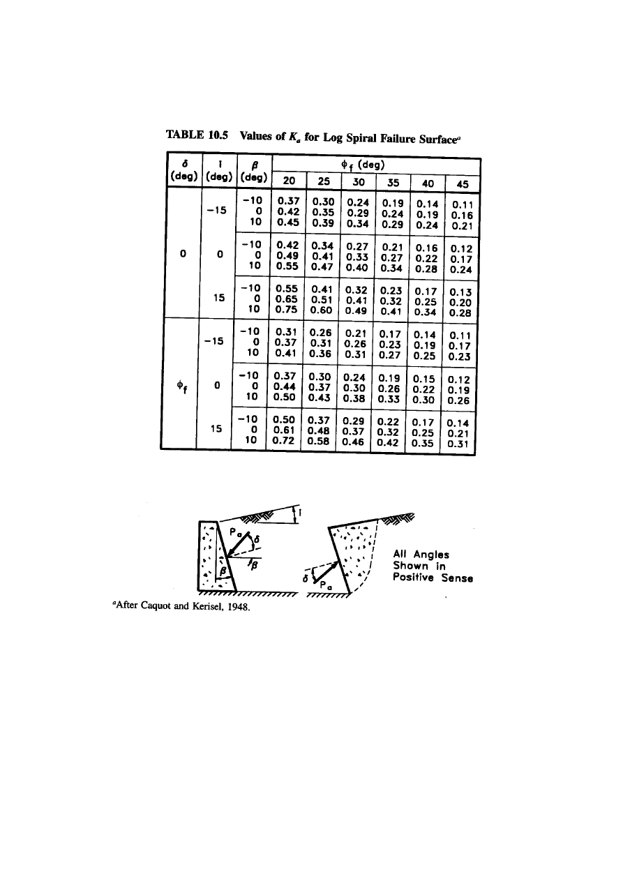
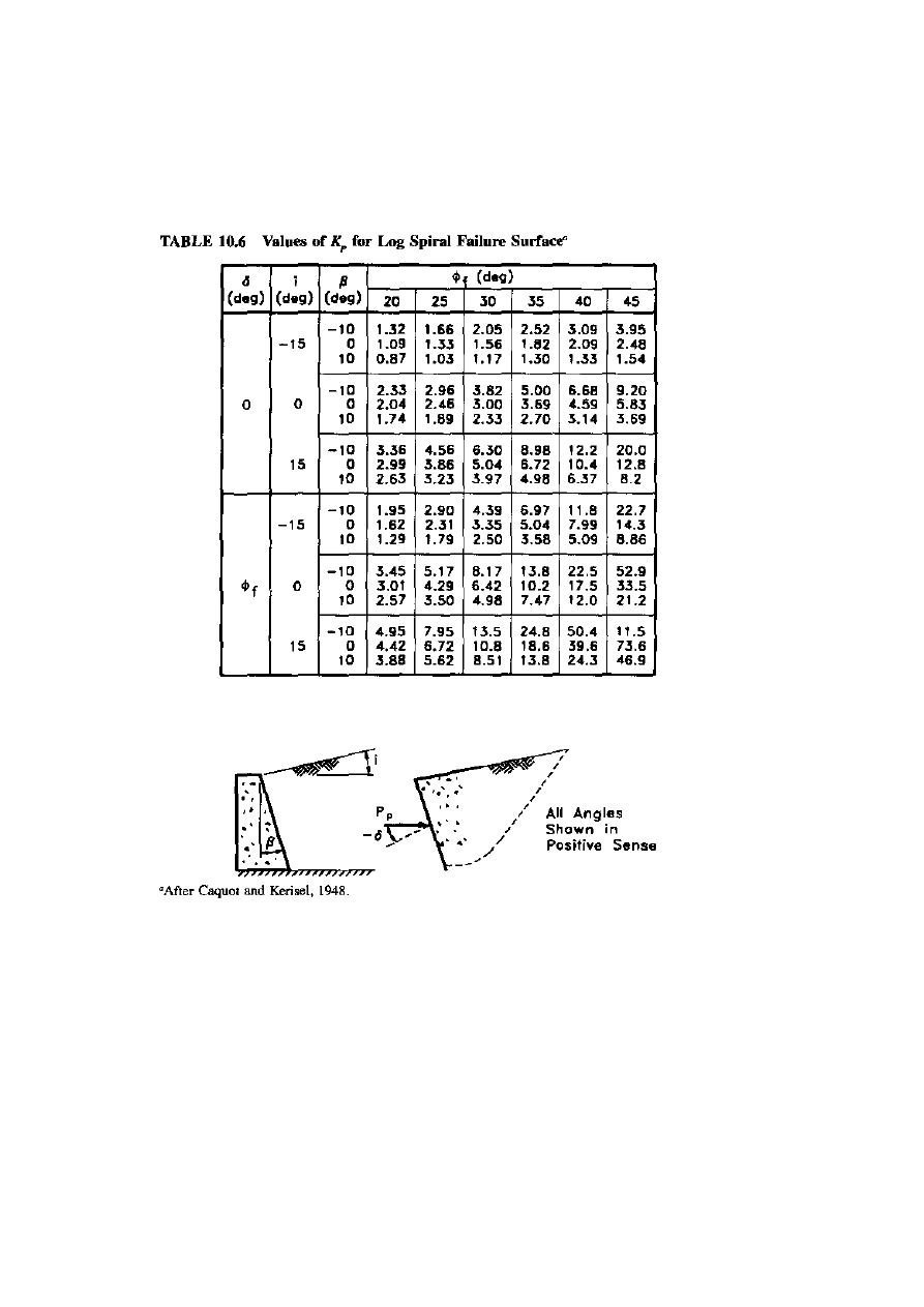
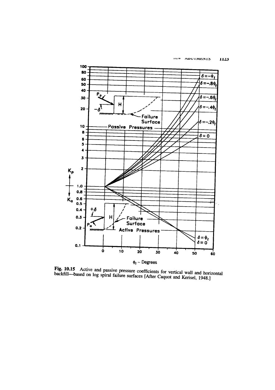
LOG SPIRAL ANALYSIS:

The failure surface in most cases is more closely approximated by a
log spiral than a straight line, as shown in

figure 10.14

.

Active and passive pressure coefficients, Ka and k

p

obtained from

analysis using log spiral surfaces are listed in

tables 10.5and 10.6

(Caquot and Kerisel, 1948). Values of Ka and k

p

for walls with level

backfill and vertical stem also shown in

figure 10.15

.

These values are

also based on the log spiral analyses performed by Caquot and

Kerisel.

SELECTION OF EARTH PRESSURE COEFFICIENTS:

Selecting a proper earth pressure coefficient is essential for
successful wall design. A number of methods previously discussed can

be used to decide the magnitude of the coefficients.
A decision on what type of earth pressure coefficient should be used is
based on the direction and the magnitude of the wall movement.

The New Zealand Ministry of Works and Development

(NAMWD, 1979) has recommended the following static earth pressure

coefficients for use in design:

1. Counterfort or gravity walls founded on rock or piles: K

0.

2. Cantilever walls less than 1880-mm high founded on rock or piles:
(K

0

+ Ka)/2.

3. Cantilever walls higher than 4880-mm or any wall founded on a

spread footing: Ka.

LOCATION OF HORIZONTAL RESULTANT:

In conventional designs and analyses, the horizontal resultant is
assumed to be located

at one-third of total height from the bottom of

the wall

. However, several experimental tests performed by

researchers conclude that the resultant is applied at

0.40H to 0.45H

from the bottom of the wall

where H is the total height of the wall.

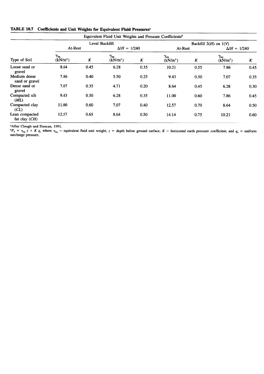
EQUIVALENT FLUID PRESSURE:

Equivalent fluid pressures provide a convenient means of estimating

design earth pressures, especially when the backfill material is a
clayey soil.
The lateral earth pressure at depth z can be expressed as

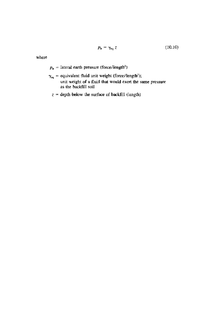
Some typical equivalent fluid unit weights and corresponding
pressure coefficients are presented in

Table 10.7.

These are

appropriate for use in designing walls up to about 6100mm in

height

.

Values are presented for at rest condition and for walls that

can tolerate movements of 1mm in 240mm, and for level and sloped

backfill.

When the equivalent fluid pressure is used in the estimation of

horizontal earth pressure it is necessary to include vertical earth
pressure acting on the wall to avoid an assumption that is too

conservative

. In the level backfill, the amount of the vertical earth

pressure acting on the wall can be taken as much as 10% of the soil
weight.

Effect of Surcharges:

When vertical loads act on a surface of the backfill near a retaining

wall or an abutment, the lateral and vertical earth pressure used for
the design of the wall should be increased.

Uniform Surcharge Load:

A surcharge load uniformly distributed over a large ground surface
area increases both the vertical and lateral pressures. The increase in

the vertical pressure, ∆P

v

is the same as the applied surcharge

pressure, q

s

. that is,

∆Pv = q

s

and the amount of increase in the lateral pressure, ∆P

h

is

∆P

h

= kq

s

Where

k = an earth pressure coefficient (dimensionless)

k = ka for active pressure

k = k

0

for at-rest condition

k = k

p

for passive pressure

Because the applied area is infinitely large, the increases in both

vertical and horizontal pressures are constant over the height of the

wall. Therefore, the horizontal resultant force due to a surcharge load

is located at mid height of the wall.

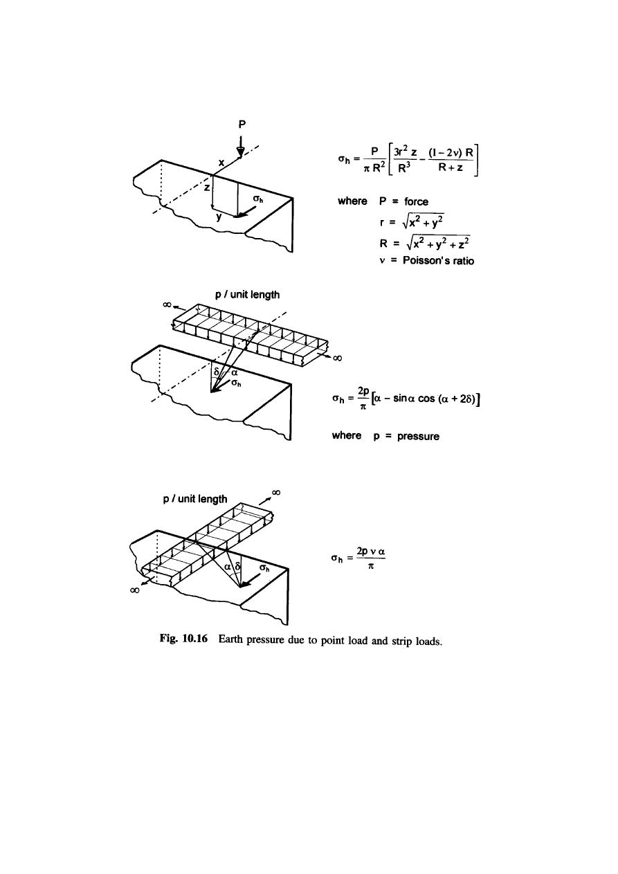
Point Load and Strip Loads:

The theory of elasticity can be used to estimate the increased earth
pressures induced by various types of surcharge loads.

Equations for earth pressures due to point load and strip loads are
presented in

Figure 10.16

.

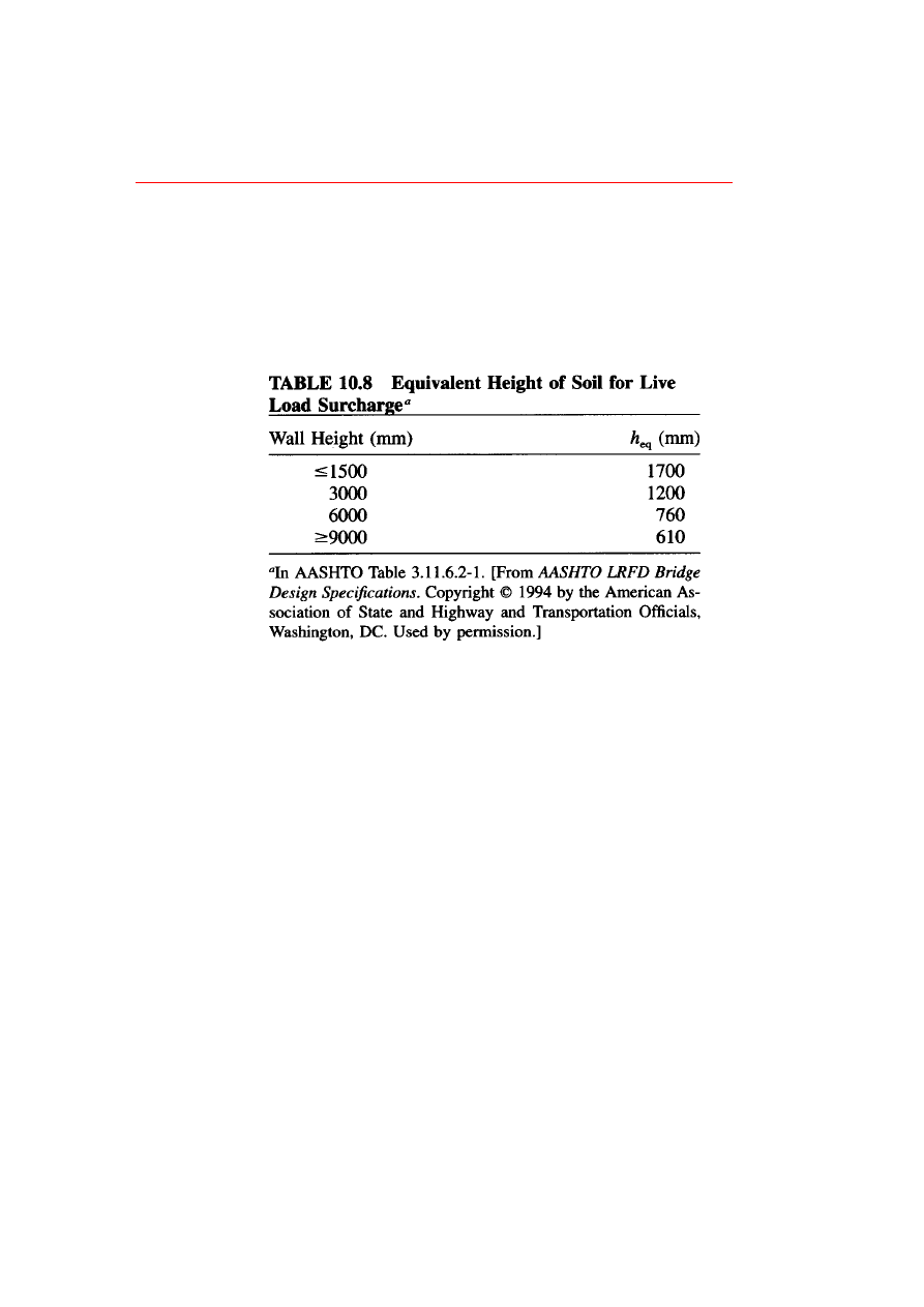
EQUIVALENT HEIGHT OF SOIL FOR LIVE LOAD SURCHARGE:

In the AASHTO (1994) LRFD Bridge Specifications, the live load
surcharge, LS, is specified in terms of an equivalent height of soil, h

eq

,

representing the vehicular loading. The values specified for h

eq

with

the height of the wall and are given in

Table 10.8

.

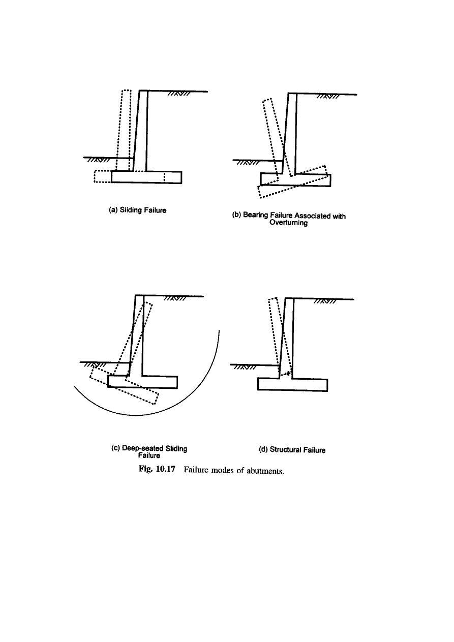
DESIGN REQUIREMENTS FOR ABUTMENTS

Failure Modes for Abutments

:

Abutments are subject to various limit states or types of failure, as

illustrated in

figure 10.17.

Failures can occur within soils or the

structural members.

i)

Sliding failure occurs when the lateral earth pressure
exerted on the abutment exceeds the frictional sliding

capacity of the foundation.

ii)

If the bearing pressure is larger than the capacity of the
foundation soil or rock, bearing failure results.

iii)

Deep-seated sliding failure may develop in clayey soil.

iv)

Structural failure also should be checked.

BASIC DESIGN CRITERIA FOR ABUTMENTS:

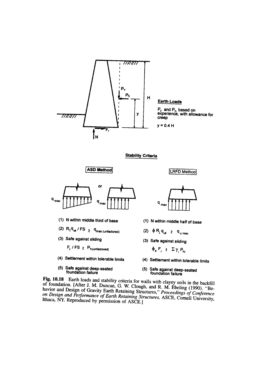
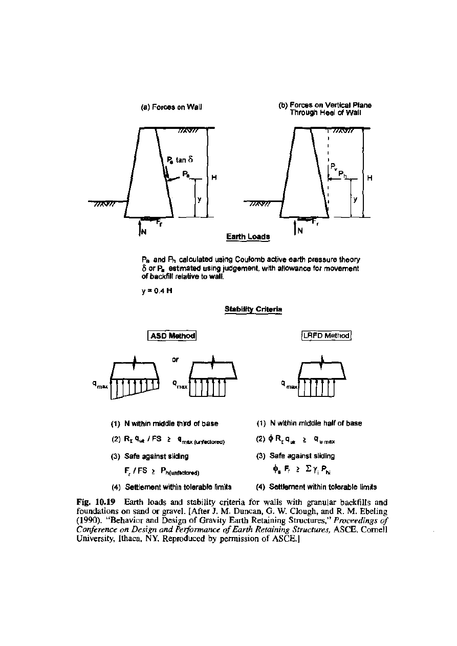
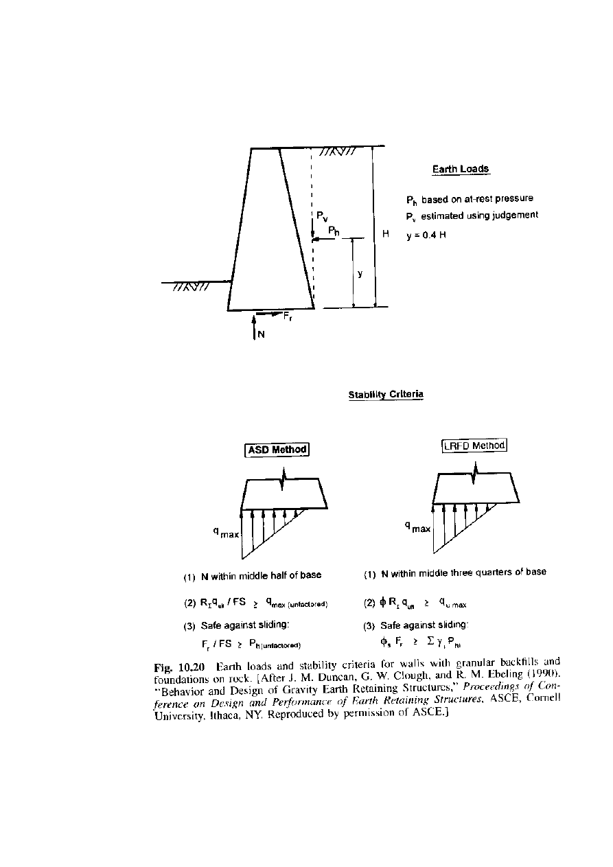
For design purposes, abutments on spread footings can be classified

into three categories (Duncan et al 1990).
1. Abutment with clayey soils in the backfill or foundations.
2. Abutment with granular backfill and foundations of sand or gravel.

3. Abutment with granular backfill and foundations on rock.
For each category, design procedures and stability criteria for the

ASD method and the LRFD method are summarized in

Figures 10.18-

10.20

.

PROCEDURE FOR DESIGN OF

ABUTMENTS:

A series of steps must be followed to obtain a satisfactory design.

STEP 1:

SELECT PRELIMINARY PROPORTIONS OF THE WALL.

STEP 2:

DETERMINE LOADS AND EARTH PRESSURES

.

STEP 3:

CALCULATE

MAGNITUDE OF REACTION FORCES ON BASE

.

STEP 4:

CHECK STABILITY AND SAFETY CRITERIA

a. Location of normal component of reactions

.

b. Adequacy of bearing pressure.

c. Safety against sliding.

STEP 5:

REVISE PROPORTIONS OF WALL AND REPEAT STEPS 2-4 UNTIL

STABILITY CRITERIA IS SATISFIED AND THEN CHECK

a. Settlement within tolerable limits

.

b. Safety against deep-seated foundation failure.

STEP 6:

IF PROPORTIONS BECOME UNRESONABLE, CONSIDER A

FOUNDATION SUPPORTED ON DRIVEN PILES OR DRILLED SHAFTS.

STEP 7:

COMPARE ECONOMICS OF COMPLETED DESIGN WITH OTHER

SYSTEMS.

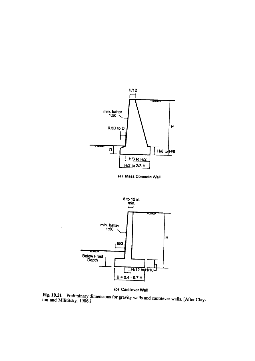
STEP 1:

SELECT PRELIMINARY PROPORTIONS OF THE WALL.

figure 10.21

shows commonly used dimensions for a gravity-retaining

wall and a cantilever wall. These proportions can be used when scour

is not a concern to obtain dimensions for a first trial of the abutment.

STEP 2:

DETERMINE LOADS AND EARTH PRESSURES.

Design loads for abutments are obtained by using group load

combinations described in Tables 3.1 and 3.2. Methods for calculating

earth pressures exerted on the wall are discussed in section 10.4.5.the
use of equivalent fluid pressures presented in table 10.7 gives
satisfactory earth pressures if conditions are no unusual.

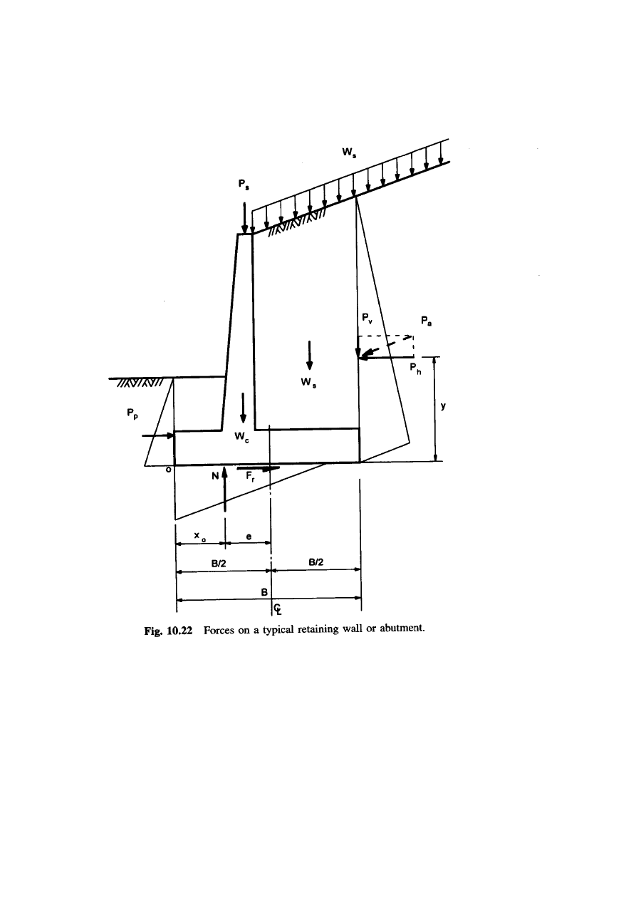
STEP 3:

CALCULATE

MAGNITUDE OF REACTION FORCES ON BASE

.

Figure 10.22

illustrates a typical cantilever wall subjected to

various loads causing reaction forces which are normal to the base
(N) and tangent to the base (Fr). These reaction forces are determined

by simple static for each load combination being investigated.

STEP 4:

CHECK STABILITY AND SAFETY CRITERIA

a. Location of normal component of reactions

.

b. Adequacy of bearing pressure.

c. Safety against sliding.

1. The location of the resultant on the base is determined by

balancing moments about the toe of the wall. The criteria for
foundation on soil for the location of the resultant is that

“it must lie within the middle half for LRFD (Figs. 10.18 and 10.19). “

This criterion replaces the check on the ratio of stabilizing moment to
overturning moment.

For foundations on rock, the acceptable location of the resultant has a
greater range than for foundations on soil

“ Middle three quarters of

base”

As shown in

figure 10.23

,

the location of the resultant, X

0,

is obtained

by

X

0

= (Summation of moments about point o) / N

Where N = the vertical resultant force (force/length).

The eccentricity of the resultant, e, with respect to the

centerline of the base is

e = B/2 – X

0

where B = base width (length)

2. Safety against bearing failure is obtained by applying a

performance factor to the ultimate bearing capacity in the LRFD
method. The ultimate BC can be calculated from the in-situ tests or

semiemperical procedures.
Safety against bearing failure is checked by

φRi qult ≥ q

umax

qult = ultimate BC (force/length)

R

I

= reduction factor due to inclined loads = (1 – Hn/Vn)

3

Hn = unfactored horizontal force

Vn = unfactored vertical force

φ = performance or resistance factor

qmax = maximum bearing pressure due to factored loads

(force/length

2

)

Shape of Bearing Pressure Distribution:

The resultant, N, will pass through the centered of a triangular or

trapezoidal stress distribution, or the middle of a uniformly
distributed stress block.

Maximum Bearing Pressure:

The following equations are used to compute the max. soil pressures,
q

umax

per unit length of a rigid footing.

For a triangular shape of bearing pressure:
When the resultant is within the middle third of base
q

umax

= Nu / B – 6 N(u) e / B2

When the resultant is outside of the

middle third of base

q

umax

= 2 N(u) / 3 Xo

For a uniform distribution of the bearing

pressure

q

umax

= N(u) / 2Xo

Where

N(u) = unfactored (factored) vertical resultant (force/length)

Xo = location of the resultant measured from toe (length)

e = eccentricity of N(u) (length)

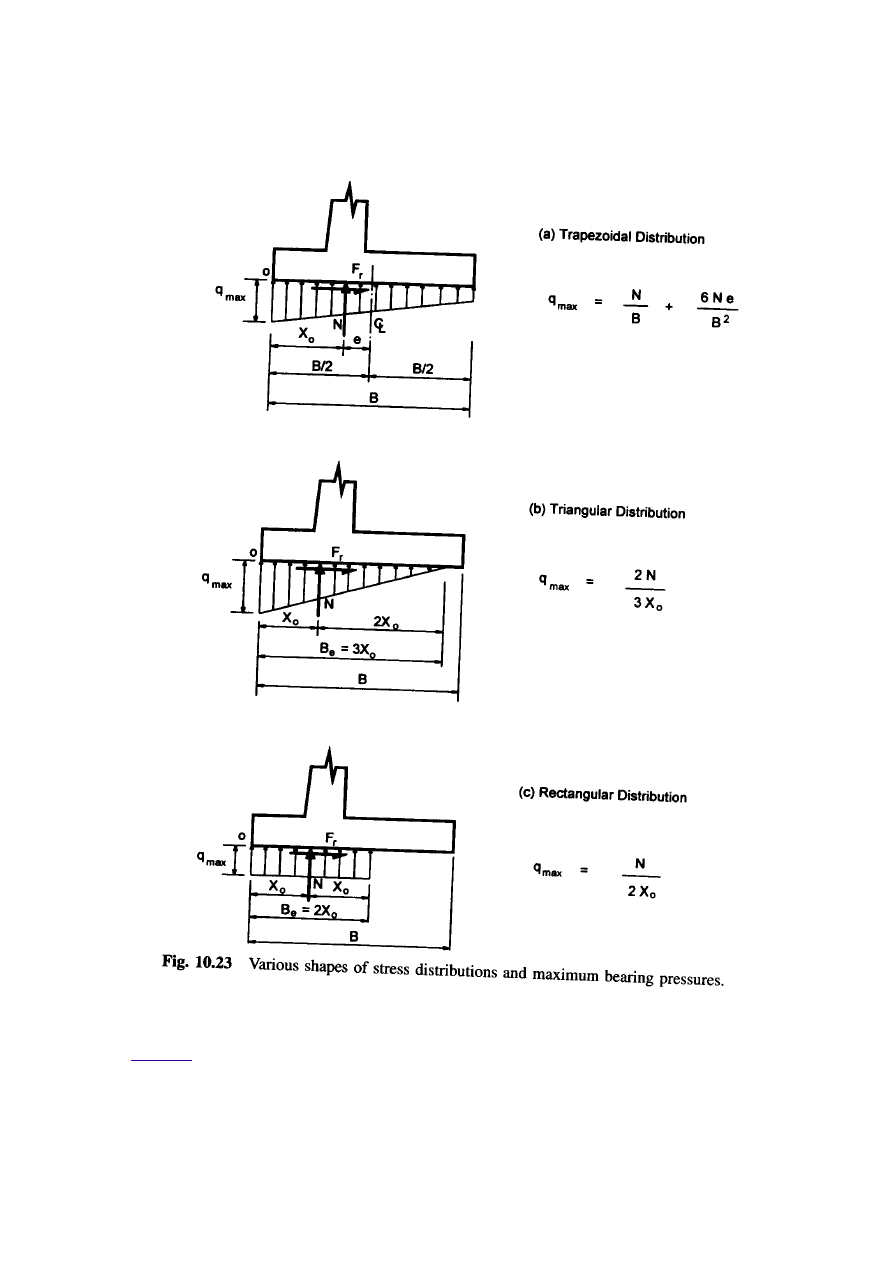
fig10.2

3

3. In the LRFD method, sliding stability is checked by
φs Fru ≥ ∑γ

i

P

hi

where

φs = performance factor for sliding

(values given in tab 10.2)

Fru =

N(u)

tan

δb + c

a

Be

Nu = factored vertical resultant
δb = friction angle b/w base and soil

ca = adhesion (force /length

2

)

Be = effective length of base in compression

γ

i

= load factor for force component i

P

hi

= horizontal earth pressure force i causing sliding (force/length)

The passive earth pressure generated by the soil in front of the wall

may be included to resist sliding if it is ensured that the soil in front of
the wall will exist permanently. However, sliding failure occurs in

many cases before the passive earth pressure is fully mobilized.
Therefore, it is safer to ignore the effect of the passive earth pressure.

STEP 5:

REVISE PROPORTIONS OF WALL AND REPEAT STEPS 2-4 UNTIL

STABILITY CRITERIA IS SATISFIED AND THEN CHECK

a. Settlement within tolerable limits

.

b. Safety against deep-seated foundation failure.

When the preliminary wall dimensions are found inadequate the wall
dimensions should be adjusted by a trial an error method.

A sensitivity study done by Kim shows that the stability can be
improved by varying the location of the wall stem, the base width, and

the wall height. Some suggestions for correcting each stability or

safety problems are presented as follows:

1. Bearing failure or eccentricity criterion not satisfied

a. Increase the base width.
b. Relocate the wall stem by moving towards the heel.
c. Minimize Ph by replacing a clayey backfill with granular material or

by reducing pore water pressure behind the wall stem with a well
designed drainage system.

d. Provide an adequately designed reinforced concrete approach slab

supported at one end by the abutment so that no horizontal pressure
due to live load surcharge need be considered.

2. Sliding stability criteria not satisfied

a. Increase the base width
b. Minimize Ph as described above

c. Use an inclined base (heel side down) to increase horizontal
distance.

d. Provide an adequately designed approach slab mentioned above.

e. Use a shear key

3. Settlement and Overall Stability Check.

Once the proportions of the wall have been selected to satisfy the

bearing pressure, eccentricity, and sliding criteria then the
requirements on settlement and overall slope stability must be

checked.

a. Settlement should be checked for walls founded on

compressible soils to ensure that the predicted settlement is
less than the settlement than the wall or structure it supports

can tolerate. The magnitude of settlement can be estimated
using the methods described in the Engineering manual for
shallow foundations.

b. The overall stability of slopes with regard to the most critical

sliding surface should be evaluated if the wall is underlain by

week soil. This check is based on limiting equilibrium methods,

which employ the modified Bishop, simplified Janbu or Spenser
analysis.

STEP 6:

IF PROPORTIONS BECOME UNRESONABLE, CONSIDER A

FOUNDATION SUPPORTED ON DRIVEN PILES OR DRILLED SHAFTS.

Driven piles and drilled shafts can be used when the configuration
of the wall is unreasonable or uneconomical.

STEP 7:

COMPARE ECONOMICS OF COMPLETED DESIGN WITH OTHER

SYSTEMS.

When a design is completed, it should be compared with other
types of walls that may result in a more economical design.

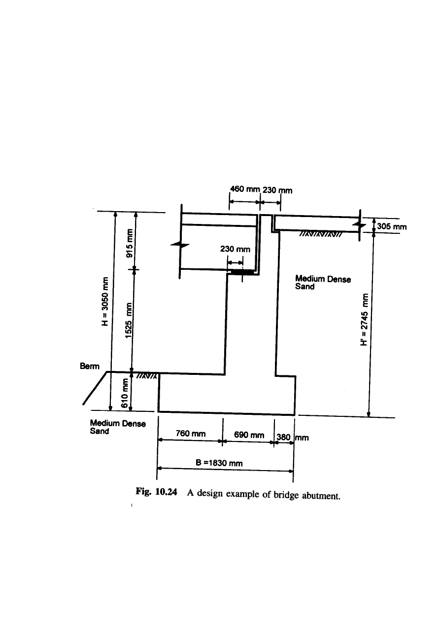
Example 10.4.7: Abutment design

Using LRFD method, the stability and safety for the abutment below is to be

checked. The abutment is found on sandy gravel with an average SPT blow count
of 22. The ultimate bearing capacity (10 tons/sft).

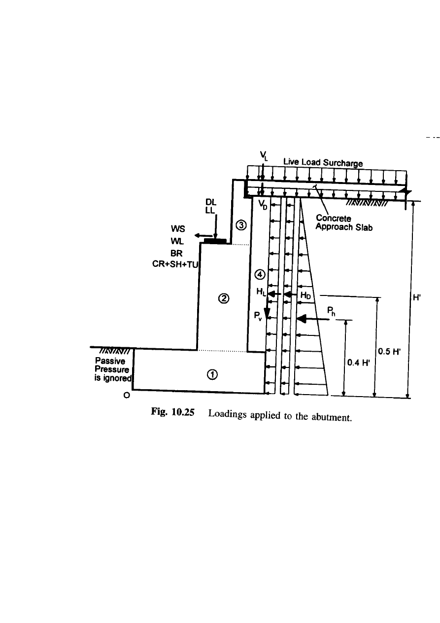
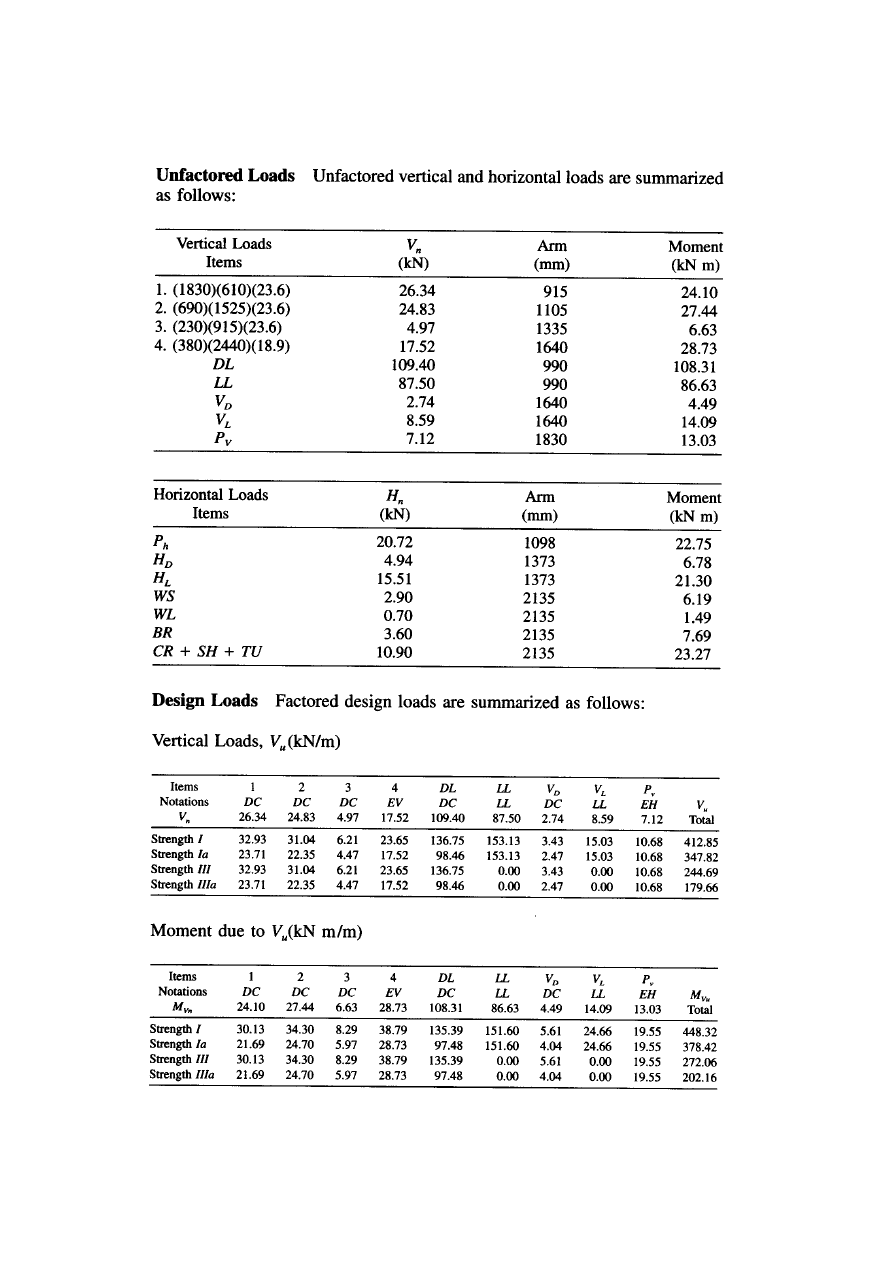
DETERMINATION OF LOADS AND EARTH PRESSURES

Loadings

: The loadings from the superstructure are given as

DL= dead load = 109.4 kN / m
LL= live load = 87.5 kN / m
WS= wind load on superstructure = 2.9 kN / m

WL = wind load on superstructure = 0.7 kN / m
BR= 3.6 kN / m

CR +SH+TU = creep, shrinkage, and temperature = 10% of DL = 10.9

kN / m

Pressures generated by the live load and dead load surcharges can be obtained as

ω

L

= h

eq

γ = 1195 mm x 18.9 kN / m

3

= 22.6 kN / m

2

ω

D

= (slab thickness) γ

c

= 305 mm x 23.6 kN / m

3

= 7.2 kN / m

2

H

L

= K ω

L

H

’

= 0.25 x 22.6 kN / m

2

x 2743 mm = 15.51 kN / m

H

D

= K ω

D

H

’

= 0.25 x 7.2 kN / m

2

x 2743 mm = 4.94 kN / m

V

L

= ω

L

* (heel width) = 22.6 kN / m

2

x 380 mm = 8.59 kN / m

V

D

= ω

D

* (heel width) = 7.2 kN / m

2

x 380 mm = 2.74kN / m

Pressures due to equivalent fluid pressure can be calculated as

P

h

= ( ½ )(EFP

h

) H

’2

= ( ½ )(5.50)(2.745)

2

= 20.72 kN / m

P

v

= ( ½ )(EFP

v

H

’2

= ( ½ )(1.89)(2.745)

2

= 7.12 kN /’ m

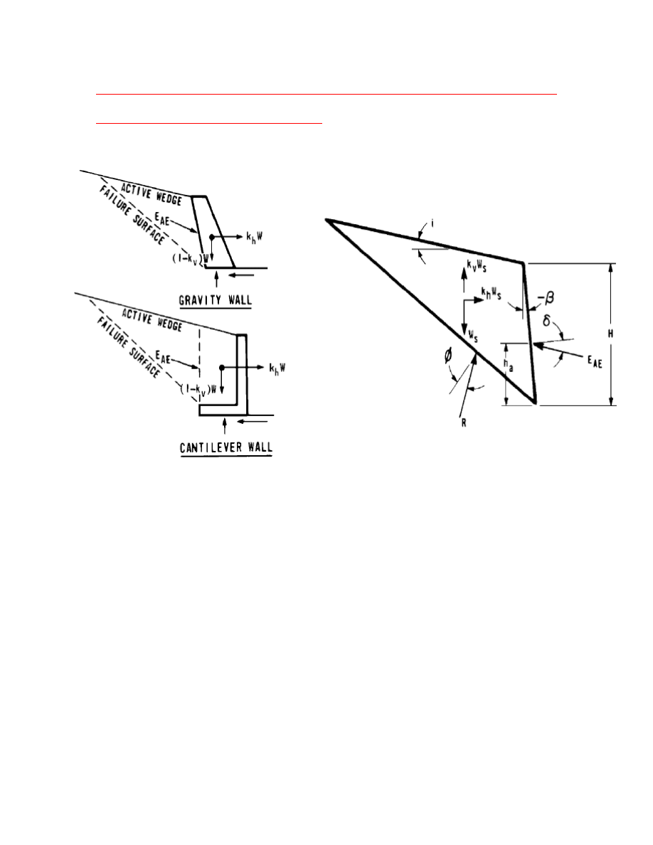
SEISMIC DESIGN OF ABUTMENTS

• The Method most commonly used for Seismic

Analysis of Free Standing Abutments is the one

Proposed in 1920’s by Mononobe and Okabe

• The method is an Extension of Coulomb Wedge

Theory, and takes into account the horizontal

and vertical forces that act on the sliding soil

wedge

• The assumptions inherent in the theory are:

ƒ

The abutment is free to yield sufficiently so

that the Active and passive conditions are

realized

ƒ

The backfill is cohesionless with internal

friction angle = φ

ƒ

The backfill is unsaturated so that

liquefaction problems do not arise

MONONOBE – OKABE THEORY FOR SEISMIC
DESIGN OF ABUTMENTS

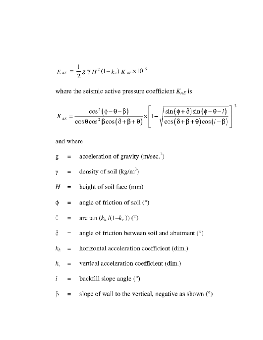
MONONOBE – OKABE THEORY FOR SEISMIC
DESIGN OF ABUTMENTS

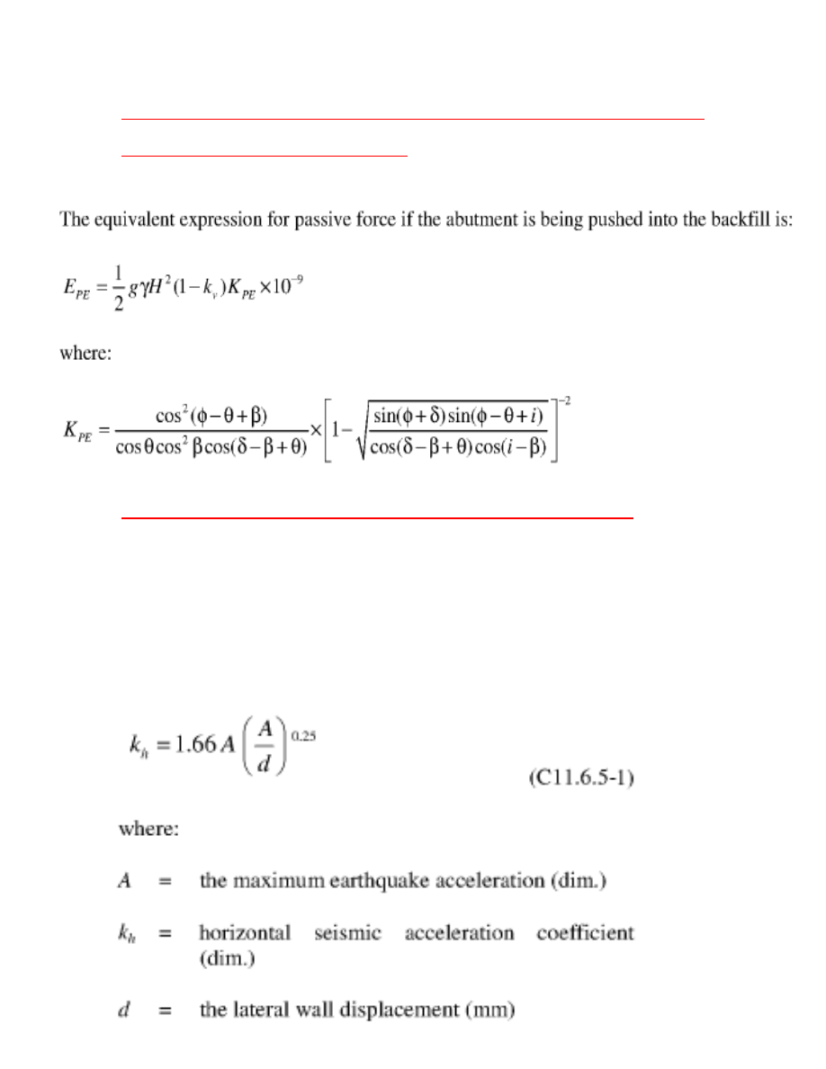
MONONOBE – OKABE THEORY FOR SEISMIC
DESIGN OF ABUTMENTS

How to Estimate Horizontal Earthquake Coefficient?

• The Seismic Force the wall is subjected to

depends upon the deformability of the wall

• If the wall is free to displace at the top, AASHTO

suggests the following relationship for

estimating EQ Coefficient

How to Estimate Horizontal Earthquake Coefficient?

• The Previous formula may be used with

confidence in Seismic Zones 1 & 2.

• For Zones 3 & 4 the advice of an earthquake

engineering expert may be sought

APPLICATION OF SEISMIC FORCE

• THE KAE and KPE given by Mononobe-Okabe

Theory contain the effect of both the Active and

Passive Pressures

• It is customary to separate the seismic force

from the Total Force as follows:

K

E

= K

AE

– K

A

Or

K

E

= K

PE

- K

P

• The Static Component of the Earth Pressure is

applied at H/3 and the Seismic Component is

applied at 0.6 H

LIMITATIONS OF MONONOBE – OKABE THEORY

• Mononobe-Okabe Theory neglects the effect of

the self weight of the wall. This should be taken

into account by estimating the seismic forces

that would be induced in the wall itself and

those transferred to the abutment from the

superstructure.