Multicommodity Flows

Lecture Outline

• Introduction
• One Commodity Flow
• Multicommodity Flows
• Types of Multicommodity Flows
• Example
• Concluding Remarks

Lecture Outline

• Introduction

• One Commodity Flow
• Multicommodity Flows
• Types of Multicommodity Flows
• Example
• Concluding Remarks

Introduction (1)

• The network structure (topology) is modeled

using various kinds of graphs and networks (graph
with additional constraints set on arcs and/or nodes)

• However, to make the model closer to a real

computer networks it is necessary to include in the
model also the flow of data (packets, bits)

• The basic tool used in research for this purpose is

theory of multicommodity flows

• The theory of multicommodity flows was developed

in the half of XX century in the context of
transport networks

Introduction (2)

• Using multicommodity flows we can in the

optimization model include network flows with

constant bit or packet rate expressed in bps

(bits per second) or pps (packets per second)

• For a transport (backbone) network carrying

the aggregated traffic consisting of numerous

single sessions we can assume that the demand

has constant rate

• The traffic network with single transmissions

characterizes with flow demand volume

changing over the time

• But modeling of such traffic is very challenging

Lecture Outline

• Introduction

• One Commodity Flow

• Multicommodity Flows
• Types of Multicommodity Flows
• Example
• Concluding Remarks

One Commodity Flow (1)

• We consider a graph G = (V, E), where V is a set of

nodes (vertices) and E is a set of edges (directed
links)

• Let A(x)={v: vV, <x,v>E} be a set of all

destination nodes of links that originate at node x

• Let B(x)={v: vV, <v,x>E} be a set of all source

nodes of links that terminates in node x

• a

ev

is 1, if link e originates at node v; 0,

otherwise

• b

ev

is 1, if link e terminates in node v; 0,

otherwise

One Commodity Flow (2)

• The commodity flow of demand volume h from

node s to node t is defined as a function f : E 

R

1

f(x,y)  0 for each <x,y>E































)

(

)

(

0

)

(

)

(

x

B

y

x

A

y

t

x

h,

s,t

x

,

s

x

h,

y,x

f

x,y

f

One Commodity Flow (3)

• Notice that

• is a difference of flow from node s to node t

leaving and entering node x

• For the source node s this value must be h

(volume)

• For the destination node t this value must be

-h

• For all other transit nodes this value must be 0











)

(

)

(

)

(

)

(

x

B

y

x

A

y

y,x

f

x,y

f

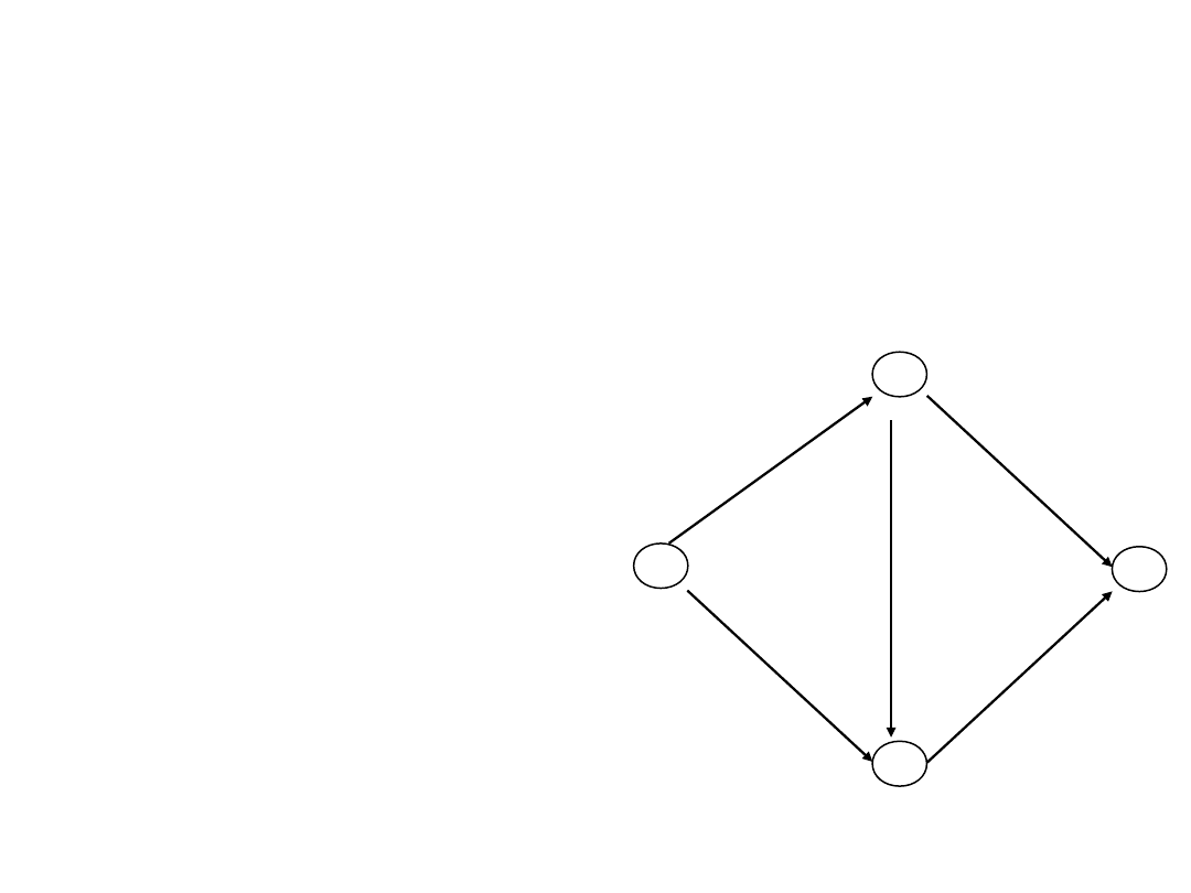
One Commodity Flow (4)

s

t

a

b

d

e

f

c

h = 3

f(s,b) = 3
f(b,f) = 3
f(f,t) = 3

3

3

3

One Commodity Flow (5)

• We assume that each link <x,y>E is assigned

with nonnegative value c(x,y), which is called

capacity of link <x,y>

• The commodity of volume h from node s to node t

is defined as a function f : E  R

1

satisfying the

following constraints

f(x,y)  c(x,y) for each <x,y>E

f(x,y)  0 for each <x,y>E































)

(

)

(

0

)

(

)

(

x

B

y

x

A

y

t

x

h,

s,t

x

,

s

x

h,

y,x

f

x,y

f

One Commodity Flow (5)

s

t

a

b

d

e

f

c

h = 3

f(s,a) = 1
f(s,b) = 2
f(a,d) = 1
f(b,f) = 2
f(d,t) = 1
f(f,t) = 2

1

1

1

2

2

2

All links
have
capacity 2

One Commodity Flow (6)

All links
have
capacity 2

s

t

a

b

d

e

f

c

h = 3

f(s,a) = 1
f(s,b) = 2
f(a,c) = 1
f(b,c) = 1
f(b,f) = 1
f(c,t) = 2
f(f,t) = 1

1

1

2

2

1

1

1

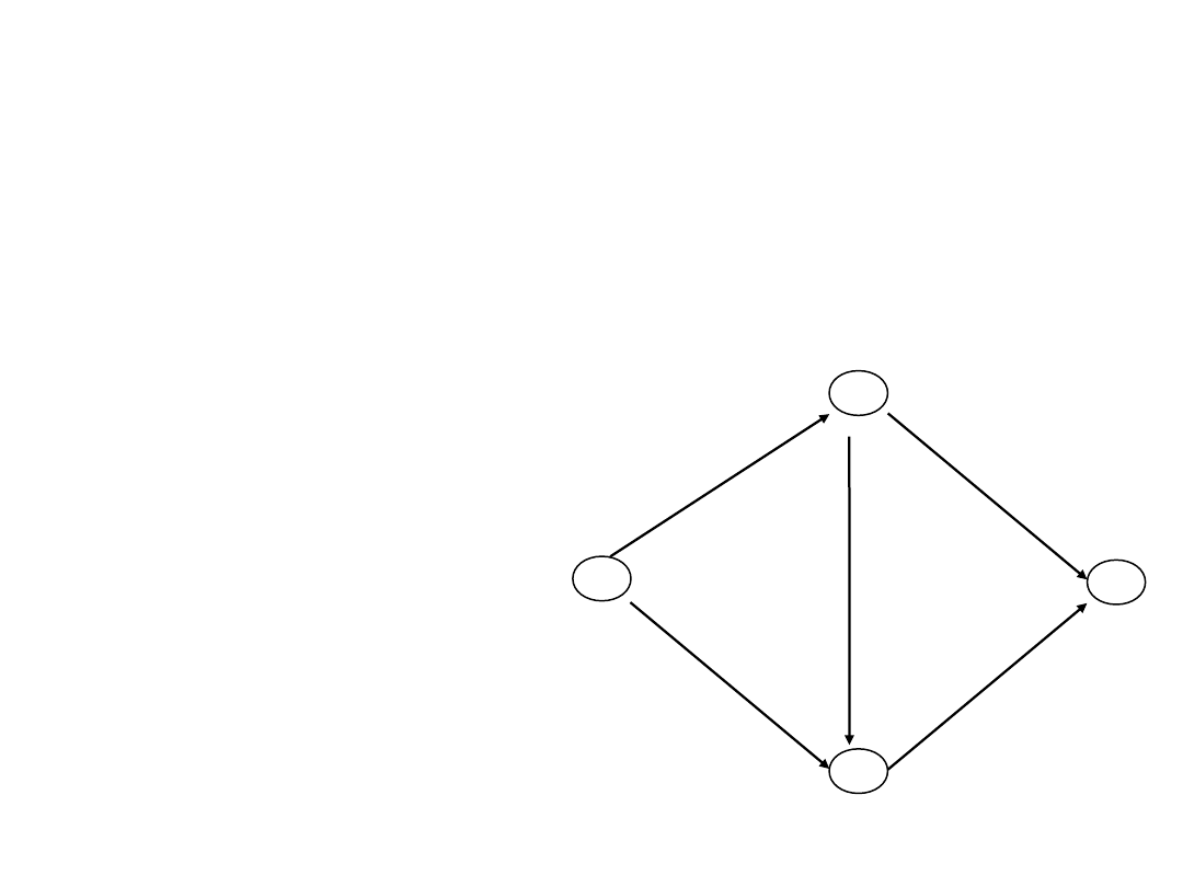
Example mcflow1.lp

Flow of one commodity (h=1) from node 1 to node 4
Minimize obj:
x12 + 3 x13 + x23 + 3 x24 + x34
Subject To
v1: x12 + x13 = 1
v2: - x12 + x23 + x24 = 0
v3: - x13 - x23 + x34 = 0
v4: - x24 - x34 = -1
Bounds
0 <= x12
0 <= x13
0 <= x23
0 <= x24
0 <= x34
End

1

4

3

2

1

3

1

3

1

Example mcflow2.lp

Flow of one commodity (h=1) from node 1 to node 4
Minimize obj:
2 x12 + 3 x13 + x23 + 2 x24 + 2 x34
Subject To
v1: x12 + x13 = 1
v2: - x12 + x23 + x24 = 0
v3: - x13 - x23 + x34 = 0
v4: - x24 – x34 = -1
Bounds
0 <= x12
0 <= x13
0 <= x23
0 <= x24
0 <= x34
End

1

4

3

2

2

3

1

2

2

Another Formulation

• v = 1,2,…,V

network nodes

• e = 1,2,…,E

links

• The commodity flow of demand volume h from

node s to node t is defined as a vector x = [x

1

,

x

2

,…,x

E

] satysifying the following contraints



e

 a

ev

x

e

 – 

e

 b

ev

x

e

 = h,   if v = s

v = 1,2,…,V



e

 a

ev

x

e

 – 

e

 b

ev

x

e

 = –h,   if v = t

v = 1,2,…,V



e

 a

ev

x

e

 – 

e

 b

ev

x

e

 = 0,  if v  s,t

v = 1,2,…,V

x

e

   0,  e = 1,2,…,E

Lecture Outline

• Introduction
• One Commodity Flow

• Multicommodity Flows

• Types of Multicommodity Flows
• Example
• Concluding Remarks

Multicommodity Flow (1)

• Multicommodity flow is defined as the average flow

of information in a particular slot of time

• The commodity (demand) is a set of packets having

the same source node and destination node

• Let h

ij

be the demand volume of traffic from node i

do node j

• All commodities (demands) are numbered from 1 to D
• Let s

d

and t

d

denote the source and destination of

demand d, respectively

• Let h

d

be the volume of demand d, i.e., h

d

= h

ij

for

i = s

d

and j = t

d

Node-Link Formulation (1)

• Multicommodity flow formulated using the node-

link notation is defined as functions

f

d

: E  R

1

   d = 1, ..., D in the following way:

f

d

(x,y)  0 for each <x,y>E































)

(

)

(

0

)

(

)

(

x

B

y

d

d

d

d

d

d

d

x

A

y

d

t

x

,

h

,t

s

x

,

s

x

,

h

y,x

f

x,y

f

Node-Link Formulation (2)

• f

d

(x,y) is the flow of commodity d in link

<x,y>

• Let f(x,y) denote the summary flow in link

<x,y>

• In computer networks usually the capacity

constraint is added to the formulation

f(x,y)  c(x,y) for each <x,y>E







D

d

d

x,y

f

x,y

f

1

)

(

)

(

Node-Link Formulation (3)

indices
v = 1,2,…,V

network nodes

e = 1,2,…,Elinks
d = 1,2,…,D

demands

constants
a

ev

= 1, if link e originates at node v; 0, otherwise

b

ev

= 1, if link e terminates in node v; 0,

otherwise

h

d

volume of demand d

Node-Link Formulation (3)

constants
s

d

source node of demand d

t

d

destination node of demand d

variables
x

ed

flow of demand d sent on link e (continuous non-

negative)

constraints


e

 a

ev

x

ed

 – 

e

 b

ev

x

ed

 = h

d

,   if v = s

d

v = 1,2,…,V

d = 1,2,…,D



e

 a

ev

x

edk

 – 

e

 b

ev

x

edk

 = –h

d

,   if v = t

d

v = 1,2,…,V

d = 1,2,…,D



e

 a

ev

x

edk

 – 

e

 b

ev

x

edk

 = 0,  if v  s

d

,t

d

v = 1,2,…,V

d = 1,2,…,D

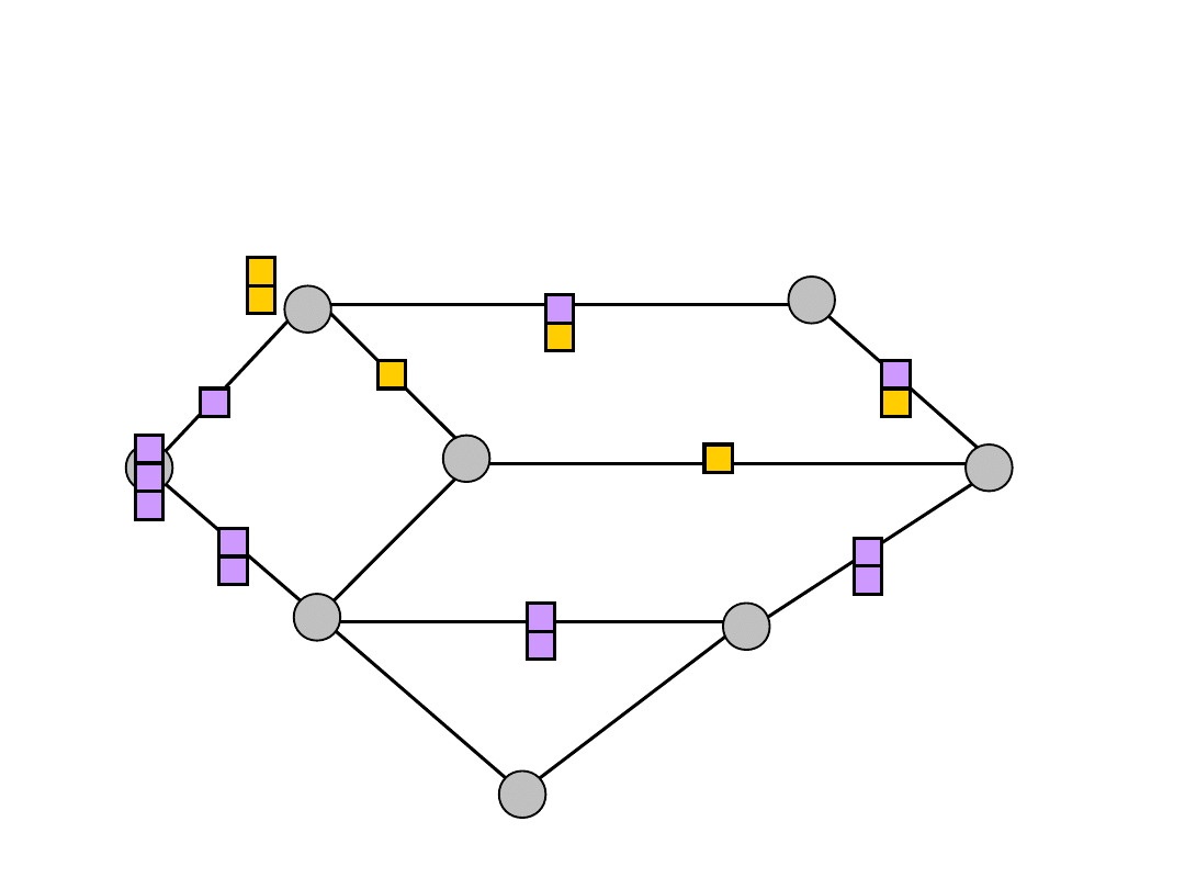
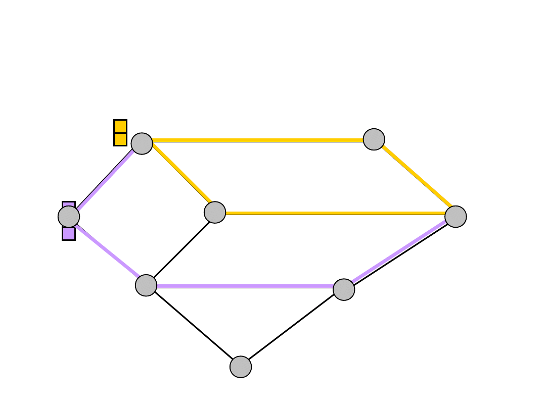
Example

s

t

a

b

d

e

f

c

h

1

= 3

All links have capacity 2

f

1

(s,a) = 1

f

1

(s,b) = 2

f

1

(a,d) = 1

f

1

(b,f) = 2

f

1

(d,t) = 1

f

1

(f,t) = 2

h

2

= 2

f

2

(a,d) = 1

f

2

(a,c) = 1

f

2

(d,f) = 1

f

2

(c,f) = 1

f(s,a) = 1
f(s,b) = 2
f(a,c) = 1
f(a,d) = 2
f(b,f) = 2
f(d,t) = 2
f(c,t) = 1
f(f,t) = 2

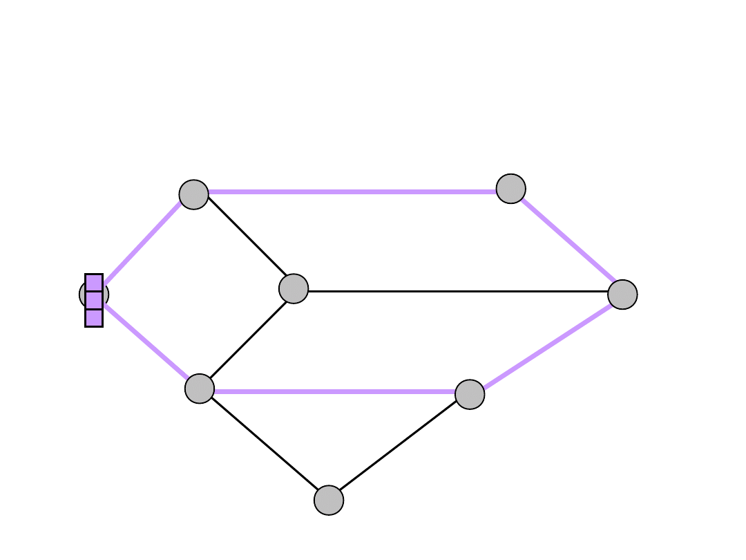
Link-Path Formulation (1)

• Multicommodity flows can be also defined using a

link-path formulation

• Let v

1

, v

2

,...,v

a

, (a > 1) be a sequence of various

nodes that <v

i

,v

i+1

> is an oriented link for each i

= 1,...,a-1

• Sequence of nodes and links v

1

, <v

1

,v

2

>, v

2

,..., v

a-

1

, <v

a-1

, v

a

>, v

a

is called a path

• For each commodity (demand) d there is a set of

candidate paths connecting nodes s

d

and t

d

(end nodes of the commodity)

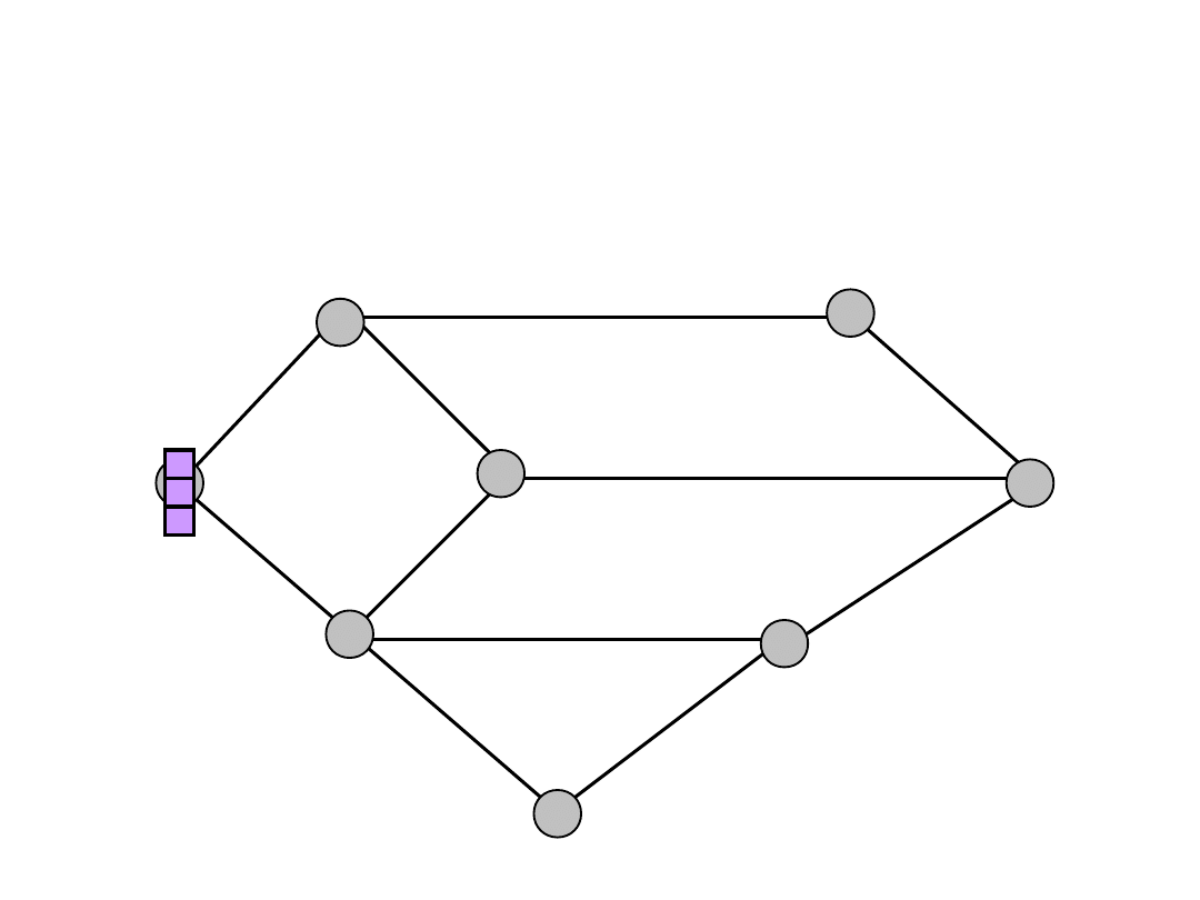
Link-Path Formulation (2)

e

s

t

a

b

d

f

c

Link-Path Formulation (3)

• Let d = 1,2, ...,D be an index of D commodities

(demands)

• Each demand is defined by the source node s

d

and destination node t

d

and demand volume h

d

• Let p = 1,2, ...,P

d

be an index of candidate paths

for demand d

• The set of candidate paths can include all possible

paths or a selected subset of all paths

• For each demand and path there is a decision

variable x

dp

(0  x

dp

 h

d

) that denotes the flow of

demand d allocated to path p

Link-Path Formulation (4)

• Variables x

dp

must satisify the following constraint



p

x

dp

= h

d

, d = 1,2,…,D.

• Constant



edp

is 1, if link e belongs to path p

realizing demand d; 0, otherwise

• f

e

denoting the summary flow in link e can be

calculated as follows

f

e

= 

d



p



edp

x

dp

e = 1,2,…,E.

Link-Path Formulation (5)

• Another formulation of x

dp

variable

• Decision variable x

dp

(0  x

dp

 1) denotes the

fraction of demand d flow allocated to path p

• Constraints



p

x

dp

= 1, d = 1,2,…,D.

f

e

= 

d



p



edp

x

dp

h

d

e = 1,2,…,E.

Link-Path Formulation (6)

• Another notation for link-path formulation
• Let P be a set of commodities numbered

p = 1, 2, ..., q with volume Q

p

• Set



p

includes indices k



p

of candidate paths

• Each path is assigned with variable

that denotes the flow of commondity p allocated
to path k

• The following constraint must be satisied

p

k

p

Q

x 



0

P

p

Q

x

p

k

p

Π

k

p









each

for

Lecture Outline

• Introduction
• One Commodity Flow
• Multicommodity Flows

• Types of Multicommodity Flows

• Example
• Concluding Remarks

Types of Multicommodity Flows

(1)

• Bifurcated flows. The commodity can be split

and sent using many different paths, e.g., IP
protocol

• Non-bifurcated (unsplittable) flows. The

whole commodity is sent along one path, e.g.,
connection oriented network techniques, e.g.
MPLS, ATM, Frame Relay

Types of Multicommodity Flows

(2)

• Link-path formulation
• Bifurcated flows. x

dp

is a continuous and non-

negative variable satisfying the following
constraint

0  x

dp

 h

d

d = 1,2,…,D p = 1,2,…,P

d

(or 0 

x

dp

 1)

• Non-bifurcated flows. x

dp

is a binary variable

satisfying the following constraint

x

dp

{0,1} d = 1,2,…,D p = 1,2,…,P

d

Types of Multicommodity Flows

(3)

• Node-link formulation
• Bifurcated flows. x

ed

is a continuous and non-

negative variable satisfying the following
constraint

0  x

ed

 h

d

d = 1,2,…,D e = 1,2,…,E (or 0  x

ed

 1)

• Non-bifurcated flows. x

ed

is a binary (integer)

variable satisfying the following constraint

x

ed

{0,1} d = 1,2,…,D e = 1,2,…,E (or x

ed

{0,h

d

})

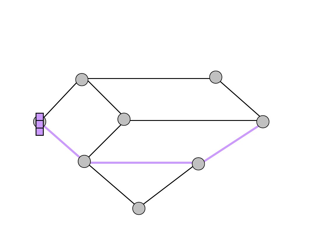
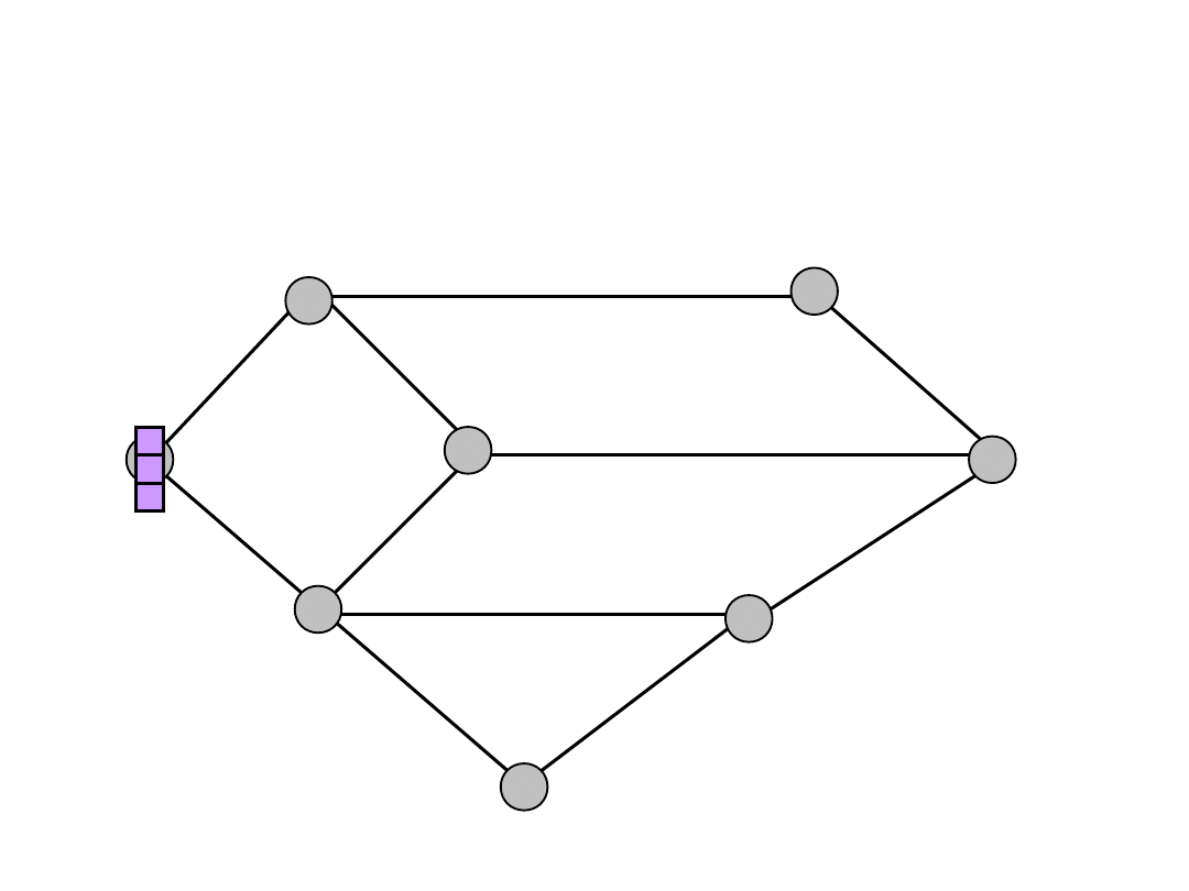
Non-bifurcated Flows

a

d

e

c

t

b

f

s

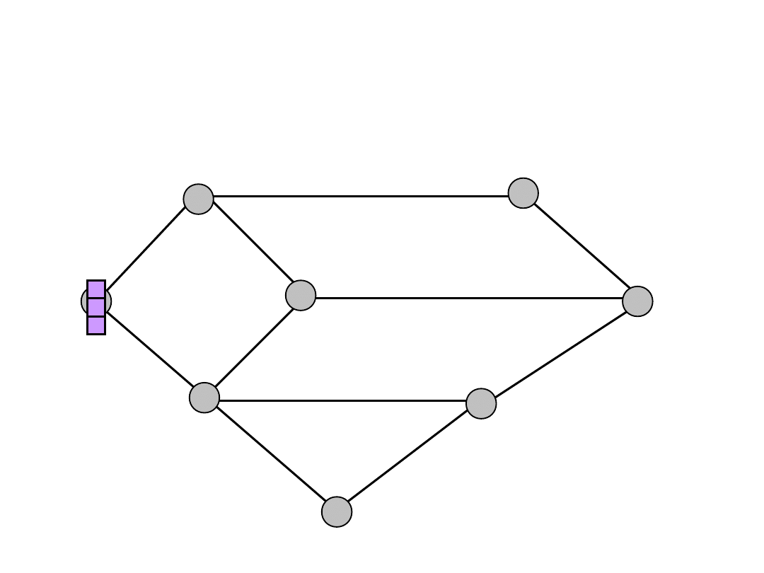
Bifurcated Flows

s

e

c

b

f

a

d

t

Lecture Outline

• Introduction
• One Commodity Flow
• Multicommodity Flows
• Types of Multicommodity Flows

• Example

• Concluding Remarks

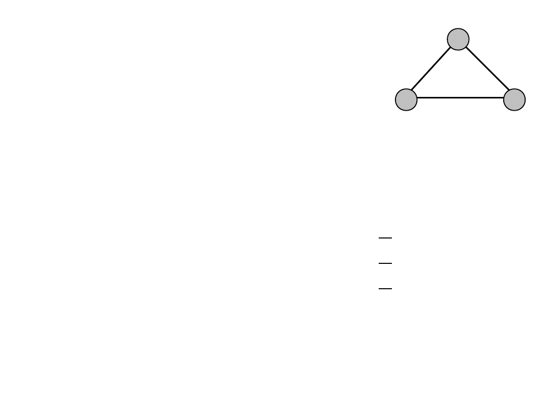
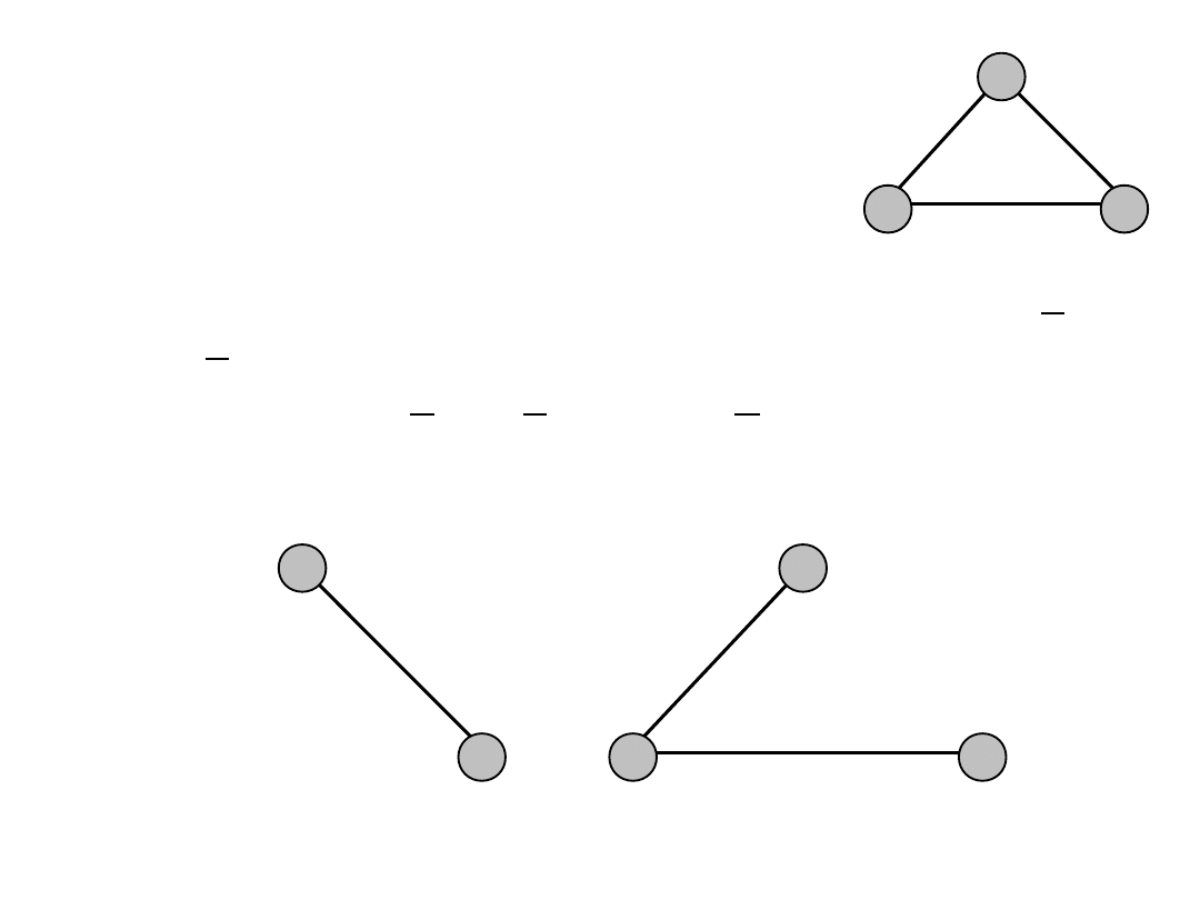
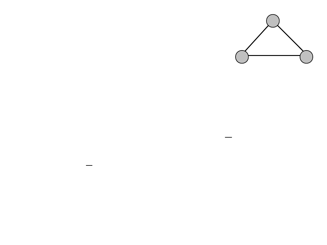
Example (1)

• Link-path notation
• The network consists of 3 nodes
• Links and demands are bi-directional

(undirected)

• Each link has cost 1
• Demand between nodes 1 and 2 is h

12

= 5

• Demand between nodes 1 and 3 is h

13

= 7

• Demand between nodes 2 and 3 is h

23

= 8

• 2 candidate paths for each demand

1

2

3

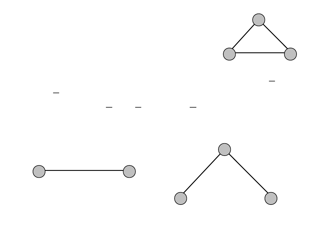
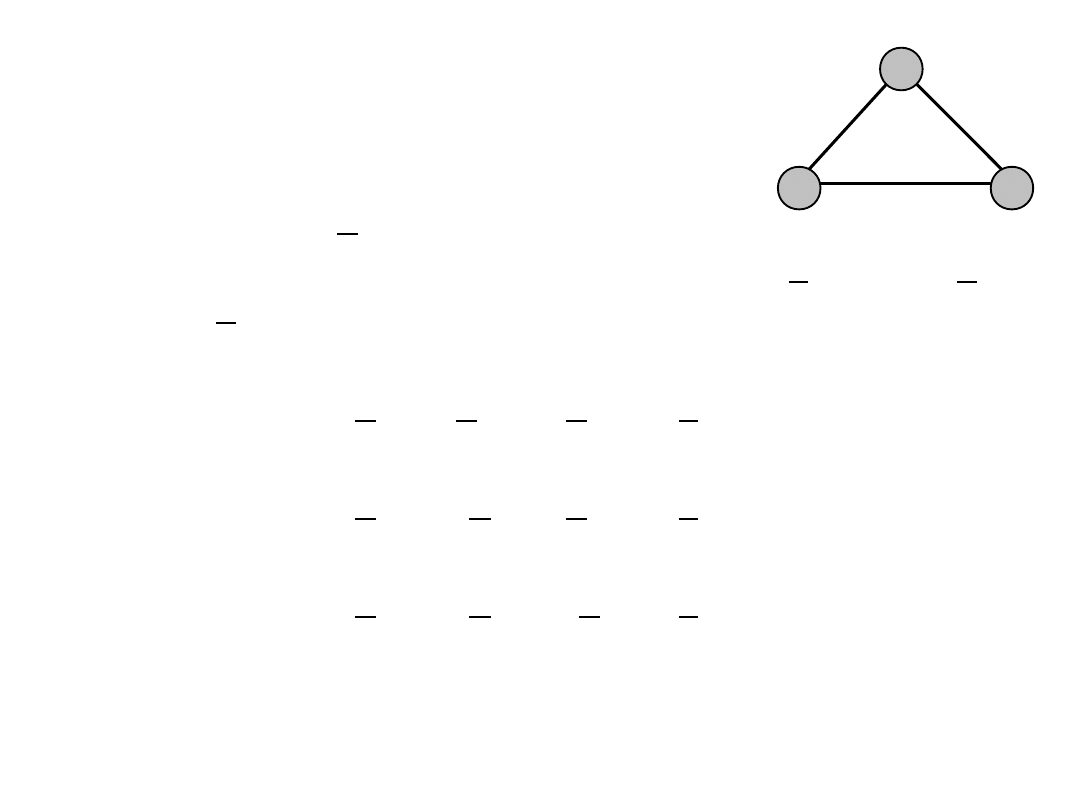
Example (2)

• Demand between nodes 1 and 2
• Path variables associated with this demand x

12

and x

132

must hold the following constraint

x

12

+ x

132

= 5 = h

12

1

2

1

2

3

1

2

3

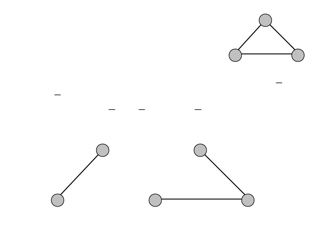
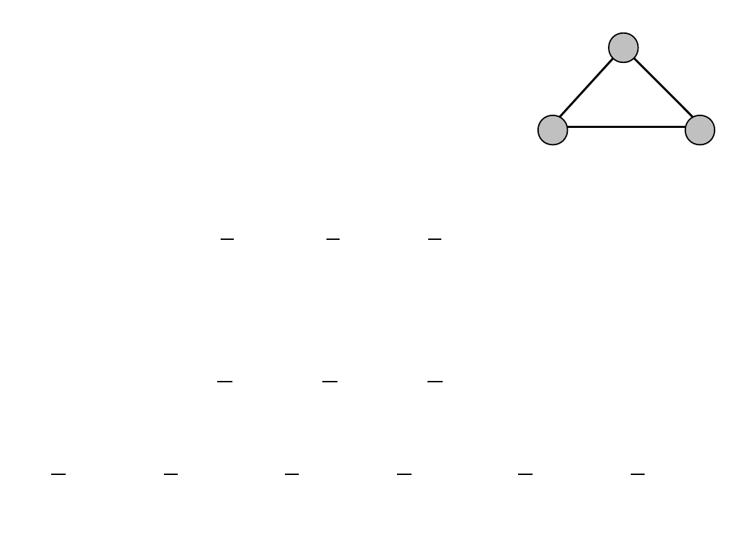
Example (3)

• Demand between nodes 1 and 3
• Path variables associated with this demand x

13

and x

123

must hold the following constraint

x

13

+ x

123

= 7 = h

13

1

3

1

2

3

1

2

3

Example (4)

• Demand between nodes 2 and 3
• Path variables associated with this demand x

23

and x

213

must hold the following constraint

x

23

+ x

213

= 8 = h

23

2

3

1

2

3

1

2

3

Example (5)

• All variables x must be non-negative
• Each edge has the following capacity c

12

= 10, c

13

= 10, c

23

= 15

• For edge 1-2 the capacity constraint is

x

12

+ x

123

+ x

213

 c

12

• For edge 1-3 the capacity constraint is

x

132

+ x

13

+ x

213

 c

13

• For edge 2-3 the capacity constraint is

x

132

+ x

123

+ x

23

 c

23

1

2

3

Example (6)

minimize

F = x

12

+ 2x

132

+ x

13

+ 2x

123

+ x

23

+ 2x

213

constraints

x

12

+ x

132

+ x

13

+ x

123

+ x

23

+ x

213

= 5 (h

12

)

x

12

+ x

132

+

x

13

+ x

123

+ x

23

+ x

213

= 7 (h

13

)

x

12

+ x

132

+ x

13

+ x

123

+

x

23

+ x

213

= 8 (h

23

)

x

12

+ x

132

+ x

13

+ x

123

+ x

23

+ x

213

 10 (c

12

)

x

12

+

x

132

+ x

13

+ x

123

+ x

23

+ x

213

 10 (c

13

)

x

12

+

x

132

+ x

13

+ x

123

+ x

23

+ x

213

 15 (c

23

)

x

12

, x

132

, x

13

, x

123

,

x

23

, x

213

 0

solution

x

*12

= 5, x

*132

= 0, x

*13

= 7, x

*123

= 0

,

x

*23

= 8

, x

*213

= 0, F

*

=

20

1

2

3

Example (7)

minimize

F = 2x

12

+ x

132

+ 2x

13

+ x

123

+ 2x

23

+ x

213

constraints

x

12

+ x

132

+ x

13

+ x

123

+ x

23

+ x

213

= 5 (h

12

)

x

12

+ x

132

+

x

13

+ x

123

+ x

23

+ x

213

= 7 (h

13

)

x

12

+ x

132

+ x

13

+ x

123

+

x

23

+ x

213

= 8 (h

23

)

x

12

+ x

132

+ x

13

+ x

123

+ x

23

+ x

213

 10 (c

12

)

x

12

+

x

132

+ x

13

+ x

123

+ x

23

+ x

213

 10 (c

13

)

x

12

+

x

132

+ x

13

+ x

123

+ x

23

+ x

213

 15 (c

23

)

x

12

, x

132

, x

13

, x

123

,

x

23

, x

213

 0

solution

x

*12

= 0, x

*132

= 5, x

*13

= 1, x

*123

= 6

,

x

*23

= 4

, x

*213

= 4, F

*

=

25

1

2

3

Example (8)

• Let link 1-2 is assigned with index 1, link 1-3 has

index 2 and link 2-3 index 3:

c

12

 c

1

,

c

13

 c

2

,

c

23

 c

3

• Let demand between nodes 1 and 2 is assigned

with index 1, demand between nodes 1 and 3 is

assigned with index 1 and between nodes 2 and 3

is assigned with index 3:

h

12

 h

1

,

h

13

 h

2

,

h

23

 h

3

• Flow variables can be defined as x

dp

, where d is the

index of demand and p is index of a candidate path:

x

12

 x

11

,

x

132

 x

12

,

x

13

 x

21

,

x

123

 x

22

,

x

23

 x

31

,

x

213



x

32

1

2

3

Example (9)

• Link-path matrix (constant



edp

)

1

2

3

link 1-2

link 1-3

link 2-3

path x

11

(1-2)

1

0

0

path x

12

(1-3-

2)

0

1

1

path x

21

(1-3)

0

1

0

path x

22

(1-2-

3)

1

0

1

path x

31

(2-3)

0

0

1

path x

32

(2-1-

3)

1

1

0

Example (10)

Using new notation we can formulate the problem

as

x

11

+ x

12

+

x

21

+ x

22

+ x

31

+ x

32

= h

1

x

11

+ x

12

+

x

21

+ x

22

+ x

31

+ x

32

= h

2

x

11

+ x

12

+ x

21

+ x

22

+ x

31

+ x

32

= h

3

x

11

+ x

12

+ x

21

+ x

22

+ x

31

+ x

32

 c

1

x

11

+

x

12

+ x

21

+ x

22

+ x

31

+ x

32

 c

2

x

11

+

x

12

+ x

21

+ x

22

+ x

31

+ x

32

 c

3

x

11

, x

12

, x

21

, x

22

,

x

31

, x

32

 0

1

2

3

Example (11)

• Node-link notation
• Directed links are used (instead bi-directional),

e.g., in place of link 1-2 we have two links 12

and 21

• Demand are also directed, e.g., h

12

is a volume

of demand from node 1 to node 2 (12)

• Variable x

13,12

denotes flow of demand 12

allocated to link 13

1

2

3

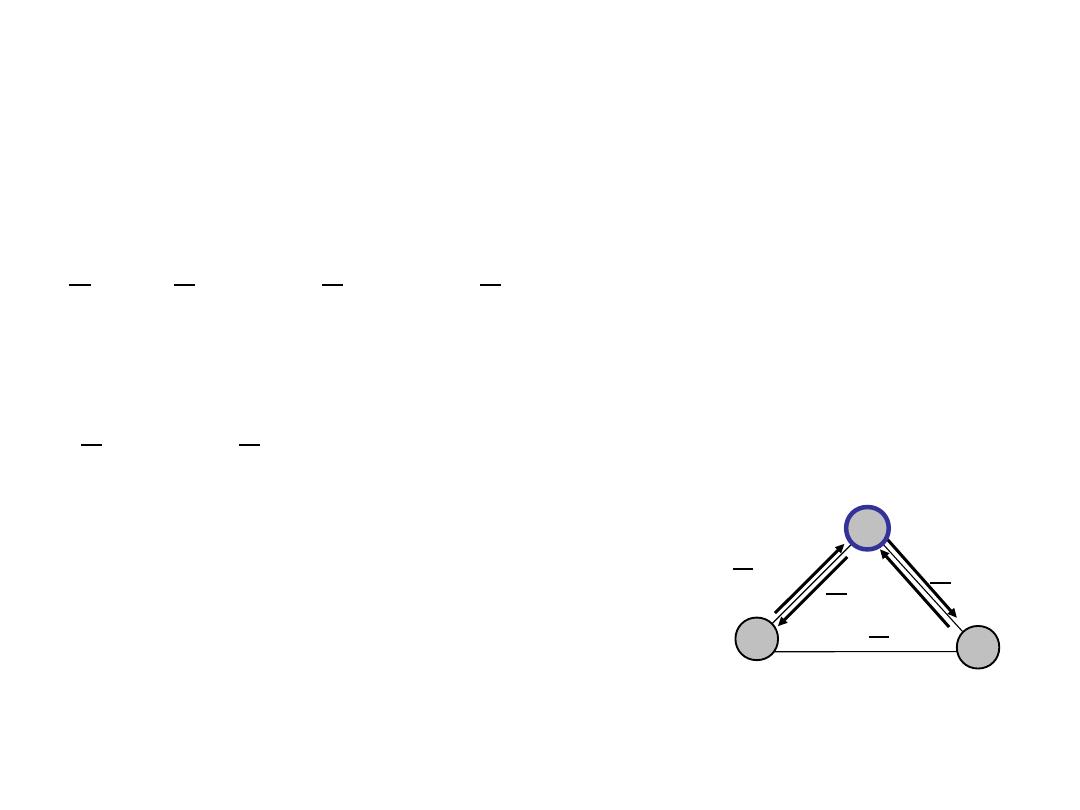
Example (12)

• Flow of demand 12 in node 1



h

12



x

21,12



x

31,12

+ x

12,12

+ x

13,12

= 0

• Since links are directed, only at most one of two

associated link can have positive flow, therefore
x

31,12

= 0 and x

21,12

= 0 and consequently we

obtain

x

12,12

+ x

13,12

= h

12

h

12

x

13,12

x

12,12

x

31,12

x

21,12

1

3

2

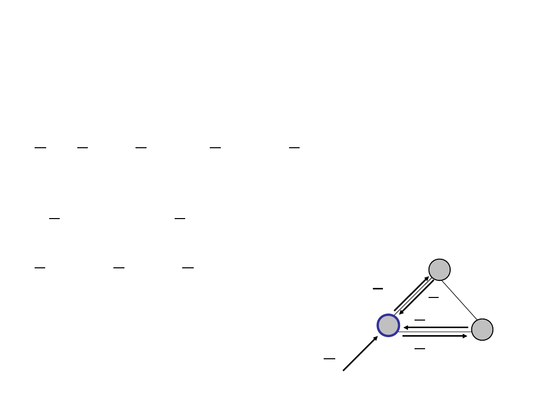
Example (13)

• Flow of demand 12 in node 3



x

13,12



x

23,12

+ x

31,12

+ x

32,12

= 0

• Node 3 is a transit node for demand 12
• Since links are directed, we can write



x

13,12

+ x

32,12

= 0

x

13,12

x

32,12

x

31,12

x

23,12

1

3

2

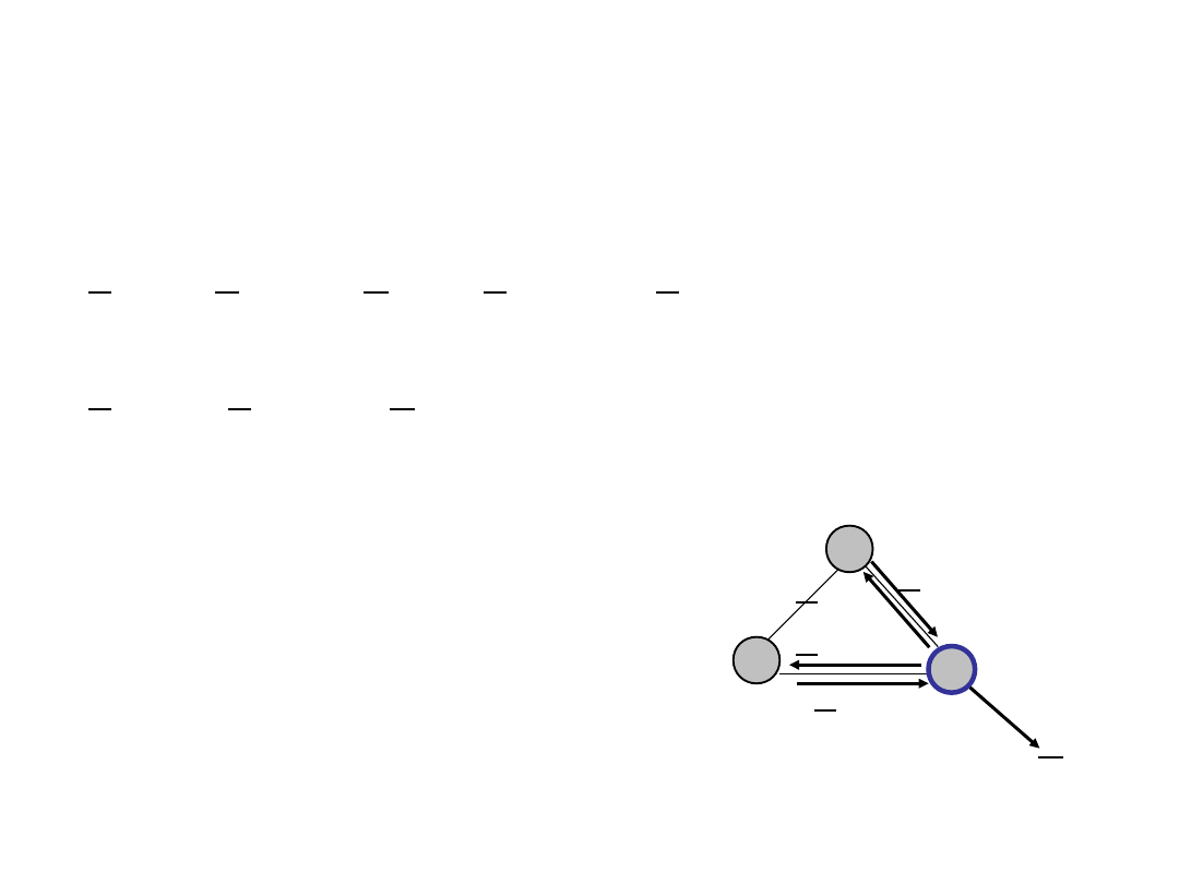
Example (14)

• Flow of demand 12 in node 2



x

12,12



x

32,12

+ h

12

+ x

21,12

+ x

23,12

= 0

• Since links are directed, we can write



x

12,12



x

32,12

=



h

12

x

32,12

x

12,12

h

12

x

21,12

x

23,12

1

3

2

Example (15)

• Link 12 can be used by demands 12 and 13,

so the capacity constraint is

x

12,12

+ x

12,13

 c

12

• For link 13 so the capacity constraint is

x

13,12

+ x

13,13

+ x

13,23

 c

13

• For all remaining links we easily can write

corresponding capacity constraints

1

2

3

Example (16)

minimize

F = x

12,12

+ x

13,12

+ x

32,12

+ x

12,13

+ x

13,13

+ x

23,13

+ x

21,23

+ x

13,23

+ x

23,23

constraints



x

12,12

+ x

13,12

+ x

32,12

+ x

12,13

+ x

13,13

+ x

23,13

+ x

21,23

+ x

13,23

+ x

23,23

= h

12

x

12,12

 x

13,12

+ x

32,12

+ x

12,13

+ x

13,13

+ x

23,13

+ x

21,23

+ x

13,23

+ x

23,23

= 0

x

12,12

+ x

13,12

 x

32,12

+ x

12,13

+ x

13,13

+ x

23,13

+ x

21,23

+ x

13,23

+ x

23,23

= h

12

x

12,12

+ x

13,12

+ x

32,12

+

x

12,13

+ x

13,13

+ x

23,13

+ x

21,23

+ x

13,23

+ x

23,23

= h

13

x

12,12

+ x

13,12

+ x

32,12

 x

12,13

+ x

13,13

+ x

23,13

+ x

21,23

+ x

13,23

+ x

23,23

= 0

x

12,12

+ x

13,12

+ x

32,12

+ x

12,13

 x

13,13

 x

23,13

+ x

21,23

+ x

13,23

+ x

23,23

= h

13

x

12,12

+ x

13,12

+ x

32,12

+ x

12,13

+ x

13,13

+ x

23,13

+

x

21,23

+ x

13,23

+ x

23,23

= h

23

x

12,12

+ x

13,12

+ x

32,12

+ x

12,13

+ x

13,13

+ x

23,13

 x

21,23

+ x

13,23

+ x

23,23

= 0

x

12,12

+ x

13,12

+ x

32,12

+ x

12,13

+ x

13,13

+ x

23,13

+ x

21,23

 x

13,23

 x

23,23

= h

23



x

12,12

+ x

13,12

+ x

32,12

+ x

12,13

+ x

13,13

+ x

23,13

+ x

21,23

+ x

13,23

+ x

23,23

 c

12

x

12,12

+ x

13,12

+ x

32,12

+ x

12,13

+ x

13,13

+ x

23,13

+

x

21,23

+ x

13,23

+ x

23,23

 c

21

x

12,12

+

x

13,12

+ x

32,12

+ x

12,13

+ x

13,13

+ x

23,13

+ x

21,23

+

x

13,23

+

x

23,23

 c

13

x

12,12

+ x

13,12

+ x

32,12

+ x

12,13

+ x

13,13

+

x

23,13

+ x

21,23

+ x

13,23

+ x

23,23

 c

23

x

12,12

+ x

13,12

+

x

32,12

+ x

12,13

+ x

13,13

+ x

23,13

+ x

21,23

+ x

13,23

+ x

23,23

 c

23

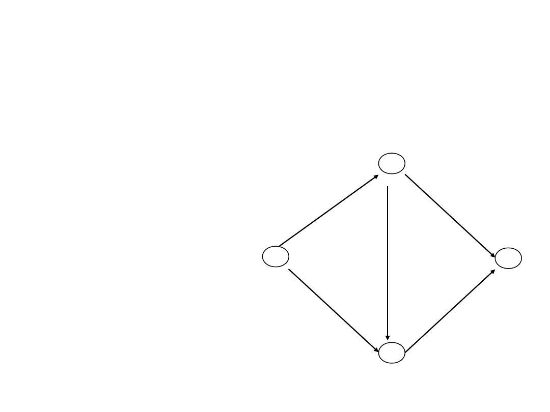
Example mcflow3.lp

Two demands: (x) nodes 1-4 and (y) nodes 2-4
Minimize obj:
x12 + 3 x13 + x23 + 3 x24 + x34 + y12 + 3 y13 + y23 + 3 y24 + y34
Subject To
v1_x: x12 + x13 = 1
v2_x: - x12 + x23 + x24 = 0
v3_x: - x13 - x23 + x34 = 0
v4_x: - x24 - x34 = -1
v1_y: y12 + y13 = 0
v2_y: - y12 + y23 + y24 = 1
v3_y: - y13 - y23 + y34 = 0
v4_y: - y24 - y34 = -1
Bounds
0 <= x12 0 <= x13 0 <= x23 0 <= x24 0 <= x34

0 <= y12 0 <= y13 0 <= y23

0 <= y24 0 <= y34

End

1

4

3

2

1

3

1

3

1

Lecture Outline

• Introduction
• One Commodity Flow
• Multicommodity Flows
• Types of Multicommodity Flows
• Example

• Concluding Remarks

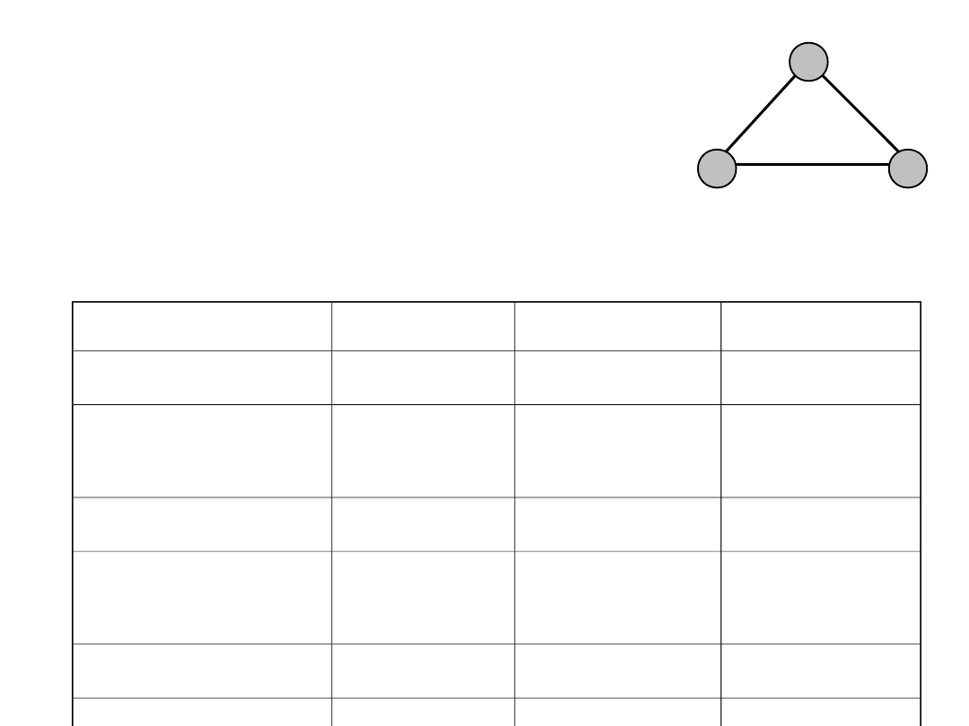
Applications of Multicommodity

Flows

Network

Nodes

Links

Flow

Information

network

People

Communicatio

n lines

News

Computer

network

Computers,

routers,

switches

Transmission

lines

Data

Railway

network

Stations,

crossings

Rail tracks

Trains

Supplying

network

Factories,

warehouse

Roads, rail

tracks

Cars, trains,

containers

Concluding Remarks

• Multicommodity flows is the basic research tool in

modeling and optimization of computer networks

• There are two basic notations of multicommodity

flows: node-link and link-path

• The selection of a particular notation depands on

the considered problem and influences the number
of decision variables and the size of the problem

• Non-bifurcated multicommodity flow problem is

integer and mostly NP-complete

Further Reading

• M. Pióro, D. Medhi, Routing, Flow, and Capacity Design in

Communication and Computer Networks, Morgan Kaufman

Publishers 2004

• R. K. Ahuja, T. L. Magnanti, and J. B. Orlin., Network Flows:

Theory, Algorithms, and Applications, Prentice Hall, 1993

• L. Ford, D. Fulkerson, Network Flows, 1962

• A. Assad, Multicommodity network flows – a survey, Networks,

Vol. 8, 1978, pp. 37–91

• J. L. Kennington, A Survey of Linear Cost Multicommodity

Networks Flows, Operations Research, Vol. 26, 1978, pp. 209–236

• M. Minoux, Multicommodity network  flow models and algorithms

in telecommunications, In: Resende, M., Pardalos, P. (eds.)

Handbook of Optimization in Telecommunications, pp. 163-184.

Springer, Heidelberg (2006)

• A. Kasprzak, Rozległe sieci komputerowe z komutacją pakietów,

Oficyna Wydawnicza Politechniki Wrocławskiej, Wrocław 1997 (in

polish)