APPLICATION NOTE

Modeling Voltage-Controlled and Temperature-Dependent
Resistors

December 2009

OVERVIEW

Analog Behavioral Modeling (ABM) can be used to model a nonlinear resistor through use of Ohms law
and tables and expressions which describe resistance. Here are some examples.

VOLTAGE-CONTROLLED RESISTOR

If a Resistance vs. Voltage curve is available, a look-up table can be used in the ABM expression. This
table contains (Voltage, Resistance) pairs picked from points on the curve. The voltage input is
nonlinearly mapped from the voltage values in the table to the resistance values. Linear interpolation is
used between table values.

Let’s say that points picked from a Resistance vs. Voltage curve are:

Voltage Resistance

0.5 25
1.0 50
2.0 100

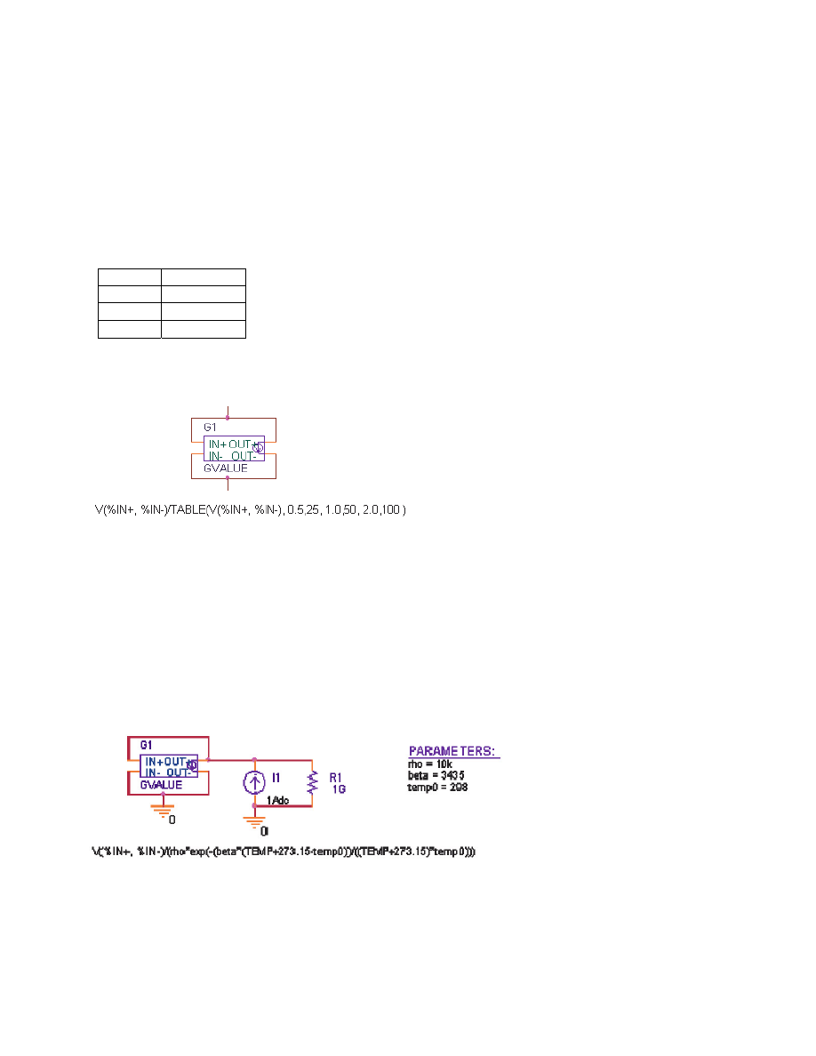
The ABM expression for this is shown in Figure 1.

Figure 1: Voltage controlled resistor using look-up table

TEMPERATURE-DEPENDENT RESISTOR

A temperature-dependent resistor (or thermistor) can be modeled with a look-up table, or an expression
can be used to describe how the resistance varies with temperature. The denominator in the expression
in Figure 2 is used to describe common thermistors. The TEMP variable in the expression is the
simulation temperature, in Celsius. This is then converted to Kelvin by adding 273.15. This step is
necessary to avoid a divide by zero problem in the denominator, when T=0 C.

NOTE:

TEMP can only be used in ABM expressions (E, G devices).

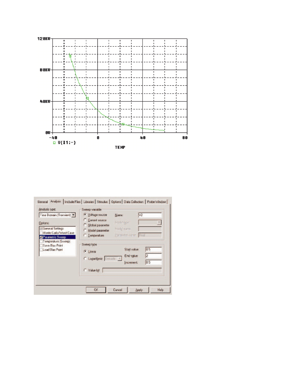
Figure 3 shows the results of a DC sweep of temperature from -40 to 60 C. The y-axis shows the
resistance or V (I1:-)/1A.

Figure 2: Temperature controlled resistor

APPLICATION

NOTE

1

Figure 3: PSpice

®

plot of Resistance vs. Temperature (current=1A)

VARIABLE Q RLC NETWORK

In most circuits the value of a resistor is fixed during a simulation. While the value can be made to change
for a set of simulations by using a Parametric Sweep to move through a fixed sequence of values, a
voltage-controlled resistor can be made to change dynamically during a simulation. This is illustrated by
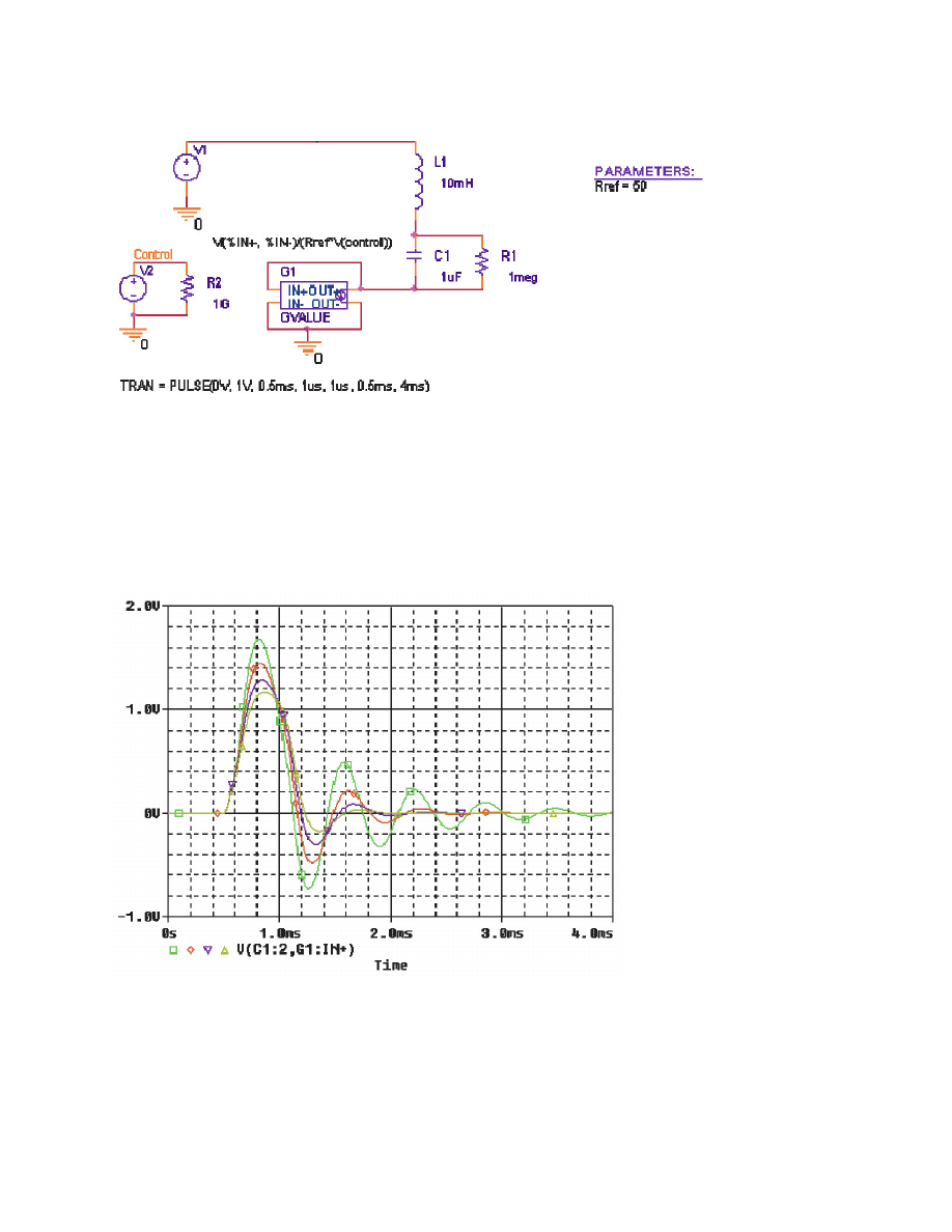
the circuit shown in Figure 5, which employs a voltage-controlled resistor.

Figure 4: Parameter sweep of control voltage

This circuit employs an external reference component that is sensed. The output impedance equals the
value of the control voltage times the reference. Here, we will use Rref, a 50 ohm resistor as our
reference. As a result, the output impedance is seen by the circuit as a floating resistor equal to the value
of V (Control) times the resistance value of Rref. In our circuit, the control voltage value is stepped from
0.5 volt to 2 volts in 0.5 volt steps; therefore, the resistance between nodes 3 and 0 varies from 25 ohms
to 100 ohms in 25 ohm-steps.

APPLICATION

NOTE

2

APPLICATION

NOTE

3

Figure 5: Variable Q RLC circuit

A transient analysis of this circuit using a 0.5 ms wide pulse will show how the ringing differs as the Q is
varied.

Using Probe, we can observe how the ringing varies as the resistance changes. Figure 6 shows the input
pulse and the voltage across the capacitor C1. Comparing the four output waveforms, we can see the
most pronounced ringing occurs when the resistor has the lowest value and the Q is greatest. Any signal
source can be used to drive the voltagecontrolled resistance. If we had used a sinusoidal control source
instead of a staircase, the resistance would have varied dynamically during the simulation.

Figure 6: Output waveforms of variable Q RLC circuit

© Copyright 2009 Cadence Design Systems, Inc. All rights reserved. Cadence, the Cadence logo, and Pspice are registered trademarks of Cadence Design Systems, Inc. All
others are properties of their respective holders.

21312 12/09 MK/DM/PDF