Exploring Economics 4e Chapter 10

C H A P T E R

O N S U M E R

H O I C E

H E O R Y

O N S U M E R

H O I C E

H E O R Y

10.1

Consumer Behavior

10.2

The Consumer’s Choice

APPENDIX:

A More Advanced Theory of Consumer
Choice

n this chapter, we discuss how individuals allocate
their income between different bundles of goods.
This decision involves trade-offs—if you buy more
of one good, you cannot afford as much of other

goods. Why do consumers buy more of a product
when the price falls and less of a product when the

price rises? How do consumers respond to rising
income? Falling income? How do we as consumers
choose certain bundles of goods with our available
budget to fit our desires? We address these questions
in this chapter to strengthen our understanding of
the law of demand.

■

95469_10_Ch10-p241-270.qxd 29/12/06 12:03 PM Page 243

244

M O D U L E 3

Households, Firms, and Market Structure

As you may recall from Chapter 4, the law of demand
is intuitive. Put simply, at a higher price, consumers
will buy less (a decrease in the quantity demanded); at
a lower price, consumers will buy more (an increase
in quantity demanded), ceteris paribus. However, the
downward-sloping demand curve has three other
explanations: (1) the income and substitution effects
of a price change, (2) the law of diminishing marginal
utility, and (3) an interpretation using indifference
curves and budget lines (in the appendix).

Let’s start with out first explanation of a downward-

sloping demand curve—the substitution and income
effects of a price change. For example, if the price of
pizza increases, the quantity of pizza demanded will fall

because some consumers might switch out of pizza
into hamburgers, tacos, burritos, submarine sandwiches,
or some other foods that
substitute for pizza.
This behavior is called
the

substitution effect

of a price change. In
addition, a price increase
for pizza will reduce
the quantity of pizza
demanded because it reduces a buyer’s purchasing
power. The buyer cannot buy as many pieces of pizza
at higher prices as she could at lower prices, which is
called the

income effect

of a price change.

The second explanation for the negative relation-

ship between price and quantity demanded is what
economists call

diminishing marginal utility.

In a

given time period, a buyer will receive less satisfaction
from each successive unit consumed. For example, a
second ice cream cone will yield less satisfaction than
the first, a third less sat-
isfaction than the second,
and so on. It follows
from diminishing mar-
ginal utility that if people
are deriving less satisfac-
tion from successive
units, consumers would
buy added units only if
the price were reduced.
Let’s now take a closer
look at utility theory.

UTILITY

To more clearly define the relationship between con-
sumer choice and resource allocation, economists
developed the concept of

utility

—a measure of the

relative levels of satis-
faction that consumers
get from the consump-
tion of goods and serv-
ices. Defining one

util

as equivalent to one
unit of satisfaction,

S E C T I O N

10.1

C o n s u m e r B e h a v i o r

■

What is the substitution effect?

■

What is the income effect?

■

Can we make interpersonal utility
comparisons?

■

What is diminishing marginal utility?

Economists conducted an experiment with rats to see how they
would respond to changing prices of different drinks (changing
the number of times a rat had to press a bar). Rats responded
by choosing more of the beverage with a lower price, showing
they were willing to substitute when the price changed. That is,
even rats seem to behave rationally—responding to incentives
and opportunities to make themselves better off.

substitution effect

a consumer’s switch to another simi-
lar good when the price of the pre-
ferred good increases

income effect

reduction in quantity demanded of
a good when its price increases
because of a consumer’s decreased
purchasing power

diminishing
marginal utility

a good’s ability to provide less satis-
faction with each successive unit
consumed

utility

a measure of the relative levels of
satisfaction consumers get from
consumption of goods and services

95469_10_Ch10-p241-270.qxd 29/12/06 12:03 PM Page 244

C H A P T E R 1 0

Consumer Choice Theory

245

economists can indi-
cate relative levels
of consumer satisfac-
tion that result from

alternative choices.

For example, for a java junkie who wouldn’t dream
of starting the day without a strong dose of
caffeine, a cup of coffee might generate 150 utils
of satisfaction while a cup of herb tea might only
generate 10 utils.

Inherently, utility varies from individual to indi-

vidual depending on specific preferences. For exam-
ple, Jason might get 50 utils of satisfaction from
eating his first piece of apple pie, while Brittany may
only derive 4 utils of satisfaction from her first piece
of apple pie.

In fact, a whole school of thought called utilitar-

ianism, based on utility theory, was developed by
Jeremy Bentham. Bentham believed that society

should seek the greatest happiness for the greater
number (See Bentham’s biography below.).

UTILITY IS A PERSONAL MATTER

Economists recognize that it is not really possible to
make interpersonal utility comparisons. That is, they
know that it is impossible to compare the relative sat-
isfactions of different persons. The relative satisfactions
gained by two people drinking cups of coffee, for
example, simply cannot be measured in comparable
terms. Likewise, although we might be tempted to
believe that a poorer person would derive greater util-
ity from finding a $100 bill than would a richer person,
we should resist the temptation. We simply cannot
prove it. The poorer person may be “monetarily” poor
because money and material things are not important
to her, and the rich person may have become richer
because of his lust for the things money can buy.

util

one unit of satisfaction

g r e a t e c o n o m i c t h i n k e r s

Jeremy Bentham (1748–1832)

Jeremy Bentham was born in London in 1748. He was a gifted child, reading his-
tory and other “serious” books at age 3, playing the violin at age 5, and study-
ing Latin and French when he was only 6. At 12, he entered Queens College,
Oxford, where he studied law. In his late teens, Bentham decided to concen-
trate on his writings. With funding provided by his father, he wrote a series of
books on philosophy, economics, and politics. He would often write for 8 to
12 hours a day, a practice that continued through his life, leaving scholars
material to compile for years to come. Most of his writings were not pub-
lished until well over a century after his death.

According to Bentham, “pain and pleasure are the sovereign masters gov-

erning man’s conduct”: People will tend to pursue things that are pleasurable
and avoid things that are painful. To this day, the rule of rational choice—
weighing marginal benefits against marginal costs—has its roots in the earlier
works of Jeremy Bentham. That is, economists predict human behavior on the
basis of people’s responses to changing incentives; people make choices on the
basis of their expected marginal benefits and their expected marginal costs.

Although Bentham was most well known for utilitarianism, a philosophy

stemming from his rational-choice ideas, he also had much to say on the sub-
jects of prison reform, religion, relief to the poor, international law, and
animal welfare. He was an ardent advocate of equality. Good humored, med-
itative, and kind, he was thought to be a visionary and ahead of his time, and
he attracted the leading thinkers of the day to his company.

Bentham died in London in 1832. He left behind a strange legacy. At his

request, his body was dissected, his skeleton padded and fully clothed, and his
head preserved in the manner of South American headhunters. He asked that

this “auto-icon,” as it is now called, be seated in a glass case at the University
College in London, and that his remains should be present at all meetings for
the board. The auto-icon is still there today, although the mummified head,
which did not preserve well, has been replaced by a wax head. The real head
became an easy target for students and one story has the head being used at
soccer practice! No one is quite sure why Bentham desired such an odd after-
life for his body; explanations range from it being a testament to an inflated
sense of self-worth to a statement about religion or a practical joke.

95469_10_Ch10-p241-270.qxd 29/12/06 12:03 PM Page 245

246

M O D U L E 3

Households, Firms, and Market Structure

TOTAL UTILITY AND MARGINAL UTILITY

Economists recognize two different dimensions of
utility: total utility and marginal utility.

Total utility

is the total amount of satisfaction derived from the
consumption of a certain number of units of a good
or service. In comparison,

marginal utility

is the

extra satisfaction generated by an additional unit of a

good that is consumed

in a particular time
period. For example,
eating four slices of
pizza in an hour might
generate a total of 28
utils of satisfaction.
The first three slices of
pizza might generate a
total of 24 utils, while
the last slice generates

only 4 utils. In this case,

the total utility of eating four slices of pizza is 28 utils,
and the marginal utility of the fourth slice is 4 utils.
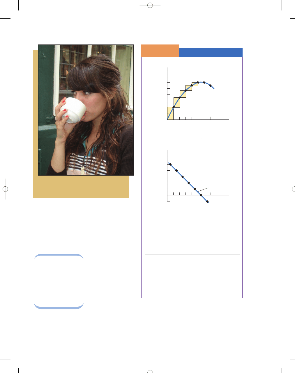
Notice in Exhibit 1(a) how total utility increases as
consumption increases (we see more total utility after
the fourth slice of pizza than after the third). But

notice, too, that the increase in total utility from each
additional unit (slice) is less than the unit before,
which indicates the marginal utility. In Exhibit 1(b)
we see how the marginal utility falls as consumption
increases.

How many utils is she deriving from this cup of coffee? Can we
accurately compare her satisfaction of a cup of coffee with
another person’s?

total utility

total amount of satisfaction derived
from the consumption of a certain
number of goods or services

marginal utility

extra satisfaction generated by con-
sumption of an additional good or
service during a specific time period

Total and Marginal Utility

S E C T I O N

1 0 .1

X H I B I T

As you can see in a, the total utility from pizza
increases as consumption increases. In b marginal util-
ity decreases as consumption increases. That is, as you
eat more pizza, your satisfaction from each additional
slice diminishes.

Slices of Pizza

Total Utility

Marginal Utility

(per day)

(utils)

−2

Total
Utility

Marginal Utility

otal Utility (utils)

Mar

ginal Utility (utils)

–2

a. Total Utility

b. Marginal Utility

Pizza Slices (consumed per hour)

95469_10_Ch10-p241-270.qxd 29/12/06 12:03 PM Page 246

C H A P T E R 1 0

Consumer Choice Theory

247

DIMINISHING MARGINAL UTILITY

Although economists believe that total utility
increases with additional consumption, they also
argue that the incremental satisfaction—the marginal
utility—that results from the consumption of addi-
tional units tends to decline as consumption increases.
In other words, each successive unit of a good that is
consumed generates less satisfaction than did the pre-
vious unit. This concept is traditionally referred to as
the

diminishing marginal utility.

Exhibit 1(b)

demonstrates this graphically, where the marginal
utility curve has a negative slope.

It follows from the

law of diminishing mar-
ginal utility that as a
person uses more and
more units of a good to
satisfy a given want, the
intensity of the want,
and the utility derived
from further satisfying
that want, diminishes. Think about it: If you are starv-
ing, your desire for that first piece of pizza will be great,
but as you eat, you gradually become more and more
full, reducing your desire for yet another piece.

diminishing
marginal utility

the concept that states that as an
individual consumes more and
more of a good, each successive
unit generate less and less utility
(or satisfaction)

using what you’ve learned

Diminishing Marginal Utility

Why do most individuals take only one newspaper from covered,
coin-operated newspaper racks when it would be so easy to take

more? Do you think potato chips, candy, or sodas could be sold profitably in
the same kind of dispenser? Why or why not?

Although ethical considerations keep some people from taking
additional papers, the law of diminishing marginal utility is also

at work here. The second newspaper adds practically zero utility to most
individuals on most days, so they typically feel no incentive to take more
than one. The exception to this case might be on Sundays, when supermar-
ket coupons are present. In that instance, while the marginal utility is still
lower for the second paper than for the first, the marginal utility of the
second paper may be large enough to tempt some individuals to take addi-
tional copies.

On the other hand, if putting money in a vending machine gave access

to many bags of potato chips, candy bars, or sodas, the temptation to take
more than one might be too great for some people. After all, the potato
chip bags would still be good tomorrow. Therefore, vending machines with

foods and drinks only dispense one item at a time, because it is likely that,
for most people, the marginal utility gained from another unit of food or
drink is higher than for a second newspaper.

Dennis MacDonald/PhotoEdit

Why are newspaper racks different from vending machines?

using what you’ve learned

The Diamond-Water Paradox:
Marginal and Total Utility

“Nothing is more useful than water: but it will not purchase scarce any-
thing. . . . Diamond, on the contrary, has scarce any value in use; but a very
great quantity of other goods may frequently be had in exchange for it.”

—Adam Smith, Wealth of Nations, 1776

Use the concept of marginal utility to evaluate the social value of
water versus diamonds.

The classic diamond-water paradox is the observation that some-
times those things that are necessary for life, like water, are inex-

pensive, and those items that are not necessary for life, like diamonds, are
expensive. This paradox puzzled philosophers for centuries. The answer

(continued)

95469_10_Ch10-p241-270.qxd 29/12/06 12:03 PM Page 247

248

M O D U L E 3

Households, Firms, and Market Structure

using what you’ve learned (cont.)

lies in making the distinction between total utility and marginal utility.
The amount of total utility is indeed higher for water than for diamonds
because of its importance for survival. But price is not determined by
total utility, it is determined by marginal utility. Total utility measures the
total amount of satisfaction someone derives from a good, whereas mar-
ginal utility determines the price. Market value—the value of the last, or
marginal, unit traded—depends on both supply and demand. Thus, the
limited supply of diamonds relative to the demand generates a high price,
but an abundant supply of water relative to the demand results in a low
price. The total utility (usefulness) for water is very large compared to the
marginal utility. Because the price of water is so low, we use so much
water that the marginal utility we receive from the last glass of water is
small. Diamonds have a much smaller total utility (usefulness) relative to
water, but because the price of diamonds is so high, we buy so few dia-
monds they have a high marginal utility. Could water ever have a higher
marginal utility than diamonds? Yes, if you had no water and no dia-
monds, your first cup of water would give you a much higher marginal

value than your first cup of diamonds. Furthermore, what if diamonds
were very plentiful and water was very scarce, which would have the
higher marginal utility? In this case, water would be expensive and dia-
monds would be inexpensive.

Why is water, which is so critical to life, priced lower than diamonds
which are less useful?

PhotoDisc Green/Getty Imeges

, Inc.

S E C T I O N

C H E C K

A substitution effect occurs when a consumer switches to another similar good when the price of the preferred

good increases.

The income effect occurs when there is a reduction in quantity demanded of a good when its price increases

because of a consumer’s decreased purchasing power.

Utility is the amount of satisfaction an individual receives from consumption of a good or service.

Economists recognize that it is not possible to make interpersonal utility comparisons.

Total utility is the amount of satisfaction derived from all units of goods and services consumed. Total

utility increases as consumption increases.

Marginal utility is the change in utility from consuming one additional unit of a good

or service.

According to the law of diminishing marginal utility, as a person consumes additional units of a given

good, marginal utility declines.

What is the substitution effect of a price change?

What is the income effect of a price change?

How do economists define utility?

Why can’t interpersonal utility comparisons be made?

What is the relationship between total utility and marginal utility?

Why could you say that a millionaire gets less marginal utility from a second piece of pizza than from

the first piece, but you couldn’t say that the millionaire derives more or less marginal utility from a second

piece of pizza than someone else who has a much lower level of income?

Are you likely to get as much marginal utility from your last piece of chicken at an all-you-can-eat restaurant as at

a restaurant where you pay $2 per piece of chicken?

95469_10_Ch10-p241-270.qxd 29/12/06 12:04 PM Page 248

C H A P T E R 1 0

Consumer Choice Theory

249

WHAT IS THE “BEST” DECISION FOR CONSUMERS?

We established the fact that marginal utility dimin-
ishes as additional units of a good are acquired. But
what significance does this idea have for consumers?
Remember, consumers try to add to their own total
utility, so when the marginal utility generated by the
purchase of additional units of one good drops too
low, it can become rational for the consumer to pur-
chase other goods rather than purchase more of the
first good. In other words, a rational consumer will
avoid making purchases of any one good beyond the
point at which other goods will yield greater satisfac-
tion for the amount spent—the “bang for the buck.”

Marginal utility, then, is an important concept in

understanding and predicting consumer behavior, espe-
cially when combined with information about prices. By
comparing the marginal utilities generated by units of
the goods that they desire as well as the prices, rational
consumers seek the combination of goods that maxi-
mizes their satisfaction for a given amount spent. In the
next section, we will see how this concept works.

CONSUMER EQUILIBRIUM

To reach consumer equilibrium, consumers must allo-
cate their incomes in such a way that the marginal util-
ity per dollar’s worth of any good is the same for every
good. That is, the “bang for the buck” must be equal
for all goods at consumer equilibrium. When this goal
is realized, one dollar’s worth of additional gasoline
will yield the same marginal utility as one dollar’s
worth of additional bread or apples or movie tickets
or soap. This concept will become clearer to you as we
work through an example illustrating the forces pres-
ent when consumers are not at equilibrium.

Given a fixed budget, if the marginal utilities per

dollar spent on additional units of two goods are not
the same, you can increase total satisfaction by
buying more of one good and less of the other. For
example, assume that the price of a loaf of bread is
$1, the price of a bag of apples is $1, the marginal
utility of a dollar’s worth of apples is 1 util, and the
marginal utility of a dollar’s worth of bread is 5 utils.

In this situation, your total satisfaction can be
increased by buying more bread and fewer apples,
because bread is currently giving you greater satisfac-
tion per dollar than apples—5 utils versus 1 util, for a
net gain of 4 utils to your total satisfaction. By buying
more bread, though, you alter the marginal utility of
both bread and apples. Consider what would happen
if, next week, you buy one more loaf of bread and one
less bag of apples. Because you are consuming more
of it now, the marginal utility for bread will fall, say
to 4 utils. On the other hand, the marginal utility for
apples will rise, perhaps to 2 utils, because you now
have fewer apples.

A comparison of the marginal utilities for these

goods in week 2 versus week 1 would look something
like this:

Week 1

bread

/$1

> MU

apples

/$1

5 utils/$1

> 1 util/$1

Week 2

bread

/$1

> MU

apples

/$1

4 utils/$1

> 2 utils/$1

Notice that although the marginal utilities of bread

and apples are now closer, they are still not equal.
Because of this difference, it is still in the consumer’s
interest to purchase an additional loaf of bread rather
than the last bag of apples; in this case, the net gain
would be 2 utils (3 utils for the unit of bread added at
a cost of 1 util for the apples given up). By buying yet
another loaf of bread, you once again push further
down your marginal utility curve for bread, and as a
result, the marginal utility for bread falls. With that
change, the relative value to you of apples increases
again, changing the ratio of marginal utility to dollar
spent for both goods in the following way:

Week 3

bread

/$1

= MU

apples

/$1

3 utils/$1

= 3 utils/$1

S E C T I O N

10.2

T h e C o n s u m e r ’s C h o i c e

■

How do consumers maximize satisfaction?

■

What is the connection between the law
of demand and the law of diminishing
marginal utility?

95469_10_Ch10-p241-270.qxd 29/12/06 12:04 PM Page 249

250

M O D U L E 3

Households, Firms, and Market Structure

What this example shows is that, to achieve

maximum satisfaction—

consumer equilibrium

—

consumers have to allocate income in such a way that

the ratio of the mar-

ginal utility to the price
of the goods is equal
for all goods pur-
chased. In other words,
in a state of consumer
equilibrium,

= MU

= . . . MU

In this situation, each good provides the consumer

with the same level of marginal utility per dollar spent.

THE LAW OF DEMAND AND THE LAW
OF DIMINISHING MARGINAL UTILITY

The law of demand states that when the price of a
good is reduced, the quantity of that good
demanded will increase. But why is this the case? By
examining the law of diminishing marginal utility in
action, we can determine the basis for this relation-
ship between price and quantity demanded. Indeed,

the demand curve merely translates marginal utility
into dollar terms.

For example, let’s say that you are in consumer

equilibrium when the price of a personal-sized pizza is
$4 and the price of a hamburger is $1. Further, in
equilibrium, the marginal utility on the last pizza con-
sumed is 40 utils, and the marginal utility on the last
hamburger is 10 utils. So in consumer equilibrium,
the MU/P ratio for both the pizza and the hamburger
is 10 utils per dollar:

pizza

(40 utils)/$4

= MU

hamburger

(10 utils)/$1

Now suppose the price of the personal-sized

pizza falls to $2, ceteris paribus. Instead of the
MU/P ratio of the pizza being 10 utils per dollar, it
is now 20 utils per dollar (40 utils/$2). This calcula-
tion implies, ceteris paribus, that you will now buy
more pizza at the lower price because you are getting
relatively more satisfaction for each dollar you
spend on pizza.

pizza

(40 utils)/$2

> MU

hamburger

(10 utils)/$1

In other words, because the price of the personal-

sized pizza fell, you are now willing to purchase more
pizzas and fewer hamburgers.

using what you’ve learned

Marginal Utility

A consumer is faced with choosing between hamburgers and milkshakes
that are priced at $2 and $1, respectively. He has $11 to spend for the week.
The marginal utility derived from each of the two goods is as follows:

If you did not have a budget constraint, you would choose 5 hamburg-

ers and 5 milkshakes because you would maximize your total utility (68

= 102); that is, adding up all the marginal utilities for all hamburgers (68

utils) and all milkshakes (34 utils). And that would cost you $15; $10 for the
5 hamburgers and $5 for the 5 milkshakes. However, you can only spend $11;
so what is the best way to spend it? Remember economic decisions are
made at the margin. This idea is the best “bang for the buck” principle, we
must equalize the marginal utility per dollar spent. Looking at the table, we
accomplish this at 4 hamburgers and 3 milkshakes per week.

= MU

10/$2

= 5/$1

× P

)

+ (Q

× P

)

= $11

× $2) + (3 × $1) = $11

Marginal Utility from

Quantity of Hamburgers

Last Hamburger

Consumed Each Week

(MU

)

Marginal Utility from

Quantity of Milkshakes

Last Milkshake

Consumed Each Week

(MU

)

consumer
equilibrium

allocation of consumer income that
balances the ratio of marginal util-
ity to the price of goods purchased

95469_10_Ch10-p241-270.qxd 29/12/06 12:04 PM Page 250

C H A P T E R 1 0

Consumer Choice Theory

251

C H A P T E R 1 0

Consumer Choice Theory

i n t h e n e w s

Behavioral Economics

Today there is a growing school of economists who are drawing on a vast range
of behavioural traits identified by experimental psychologists which amount
to a frontal assault on the whole idea that people, individually or as a group,
mostly act rationally.

A quick tour of the key observations made by these psychologists would

make even Mr Spock’s head spin. For example, people appear to be dispro-
portionately influenced by the fear of feeling regret, and will often pass up
even benefits within reach to avoid a small risk of feeling they have failed.
They are also prone to cognitive dissonance: holding a belief plainly at odds
with the evidence, usually because the belief has been held and cherished for
a long time. Psychiatrists sometimes call this “denial”.

And then there is anchoring: people are often overly influenced by outside

suggestion. People can be influenced even when they know that the suggestion
is not being made by someone who is better informed. In one experiment, vol-
unteers were asked a series of questions whose answers were in percentages—
such as what percentage of African countries is in the United Nations? A wheel
with numbers from one to 100 was spun in front of them; they were then asked
to say whether their answer was higher or lower than the number on the wheel,
and then to give their answer. These answers were strongly influenced by the
randomly selected, irrelevant number on the wheel. The average guess when the
wheel showed 10 was 25%; when it showed 65 it was 45%.

Experiments show that most people apparently also suffer from status

quo bias: they are willing to take bigger gambles to maintain the status quo
than they would be to acquire it in the first place. In one common experiment,
mugs are allocated randomly to some people in a group. Those who have them
are asked to name a price to sell their mug; those without one are asked to
name a price at which they will buy. Usually, the average sales price is consid-
erably higher than the average offer price.

Expected-utility theory assumes that people look at individual decisions

in the context of the big picture. But psychologists have found that, in fact,
they tend to compartmentalise, often on superficial grounds. They then
make choices about things in one particular mental compartment without
taking account of the implications for things in other compartments.

There is also a huge amount of evidence that people are persistently, and

irrationally, over-confident. Asked to answer a factual question, then asked to
give the probability that their answer was correct, people typically overestimate
this probability. This may be due to a representativeness heuristic: a tendency
to treat events as representative of some well-known class or pattern. This gives
people a sense of familiarity with an event and thus confidence that they have
accurately diagnosed it. This can lead people to “see” patterns in data even where
there are none. A closely related phenomenon is the availability heuristic:
people focus excessive attention on a particular fact or event, rather than the big
picture, simply because it is more visible or fresher in their mind.

Another delightfully human habit is magical thinking: attributing to one’s

own actions something that had nothing to do with them, and thus assuming that
one has a greater influence over events than is actually the case. For instance, an
investor who luckily buys a share that goes on to beat the market may become

convinced that he is a skilful investor rather than a merely fortunate one. He may
also fall prey to quasi-magical thinking—behaving as if he believes his thoughts
can influence events, even though he knows that they can’t.

Most people, say psychologists, are also vulnerable to hindsight bias:

once something happens, they overestimate the extent to which they could
have predicted it. Closely related to this is memory bias: when something hap-
pens people often persuade themselves that they actually predicted it, even
when they didn’t.

Finally, who can deny that people often become emotional, cutting off

their noses to spite their faces. One of the psychologists’ favourite experi-
ments is the “ultimatum game” in which one player, the proposer, is given a
sum of money, say $10, and offers some portion of it to the other player, the
responder. The responder can either accept the offer, in which case he gets the
sum offered and the proposer gets the rest, or reject the offer in which case
both players get nothing. In experiments, very low offers (less than 20% of the
total sum) are often rejected, even though it is rational for the responder to
accept any offer (even one cent!) which the proposer makes. And yet respon-
ders seem to reject offers out of sheer indignation at being made to accept
such a small proportion of the whole sum, and they seem to get more satis-
faction from taking revenge on the proposer than in maximising their own
financial gain. Mr Spock would be appalled if a Vulcan made this mistake.

The psychological idea that has so far had the greatest impact on eco-

nomics is “prospect theory”. This was developed by Daniel Kahneman of
Princeton University and the late Amos Tversky of Stanford University. It
brings together several aspects of psychological research and differs in crucial
respects from expected-utility theory—although, equally crucially, it shares
its advantage of being able to be modelled mathematically. It is based on the
results of hundreds of experiments in which people have been asked to
choose between pairs of gambles.

What Messrs Kahneman and Tversky claim to have found is that people are

“loss averse”: they have an asymmetric attitude to gains and losses, getting less
utility from gaining, say, $100 than they would lose if they lost $100. This is not
the same as “risk aversion”, any particular level of which can be rational if con-
sistently applied. But those suffering from loss aversion do not measure risk
consistently. They take fewer risks that might result in suffering losses than if
they were acting as rational utility maximisers. Prospect theory also claims that
people regularly miscalculate probabilities: they assume that outcomes which
are very probable are less likely than they really are, that outcomes which are
quite unlikely are more likely than they are, and that extremely improbable, but
still possible, outcomes have no chance at all of happening. They also tend to
view decisions in isolation, rather than as part of a bigger picture.

Several real-world examples of how this theory can explain human deci-

sions are reported in a forthcoming paper, “Prospect Theory in the Wild”, by
Colin Camerer, an economist at the California Institute of Technology∗. Many
New York taxi drivers, points out Mr Camerer, decide when to finish work
each day by setting themselves a daily income target, and on reaching it they
stop. This means that they typically work fewer hours on a busy day than on

(continued)

95469_10_Ch10-p241-270.qxd 29/12/06 12:04 PM Page 251

252

M O D U L E 3

Households, Firms, and Market Structure

i n t h e n e w s ( c o n t . )

a slow day. Rational labour-market theory predicts that they will do the
opposite, working longer on the busy day when their effective hourly wage-
rate is higher, and less on the slow day when their wage-rate is lower. Prospect
theory can explain this irrational behaviour: failing to achieve the daily
income target feels like incurring a loss, so drivers put in longer hours to avoid
it, and beating the target feels like a win, so once they have done that, there
is less incentive to keep working.

RACING AND THE EQUITY PREMIUM

People betting on horse races back long-shots over favourites far more often
than they should. Prospect theory suggests this is because they attach too low
a probability to likely outcomes and too high a probability to quite unlikely
ones. Gamblers also tend to shift their bets away from favourites towards
long-shots as the day’s racing nears its end. Because of the cut taken by the
bookies, by the time later races are run most racegoers have lost some money.
For many of them, a successful bet on an outsider would probably turn a
losing day into a winning one. Mathematically, and rationally, this should not
matter. The last race of the day is no different from the first race of the next
day. But most racegoers close their “mental account” at the end of each racing
day, and they hate to leave the track a loser.

Perhaps the best-known example of prospect theory in action is in sug-

gesting a solution to the “equity-premium puzzle”. In America, shares have long
delivered much higher returns to investors relative to bonds than seems justi-
fied by the difference in riskiness of shares and bonds. Orthodox economists
have ascribed this simply to the fact that people have less appetite for risk than
expected. But prospect theory suggests that if investors, rather like racegoers,
are averse to losses during any given year, this might justify such a high equity
premium. Annual losses on shares are much more frequent than annual losses on
bonds, so investors demand a much higher premium for holding shares to com-
pensate them for the greater risk of suffering a loss in any given year.

A common response of believers in homo economicus is to claim that

apparently irrational behaviour is in fact rational. Gary Becker, of the
University of Chicago, was doing this long before behavioural economics came
along to challenge rationality. He has won a Nobel prize for his work, which
has often shed light on topics from education and family life to suicide, drug
addiction and religion. Recently, he has developed “rational” models of the
formation of emotions and of religious belief.

Rationalists such as Mr Becker often accuse behaviouralists of picking

whichever psychological explanation happens to suit the particular alleged
irrationality they are explaining, rather than using a rigorous, consistent sci-
entific approach. Caltech’s Mr Camerer argues that rationalists are guilty of
exactly the same error. For instance, rationalists explain away people’s fond-
ness for betting on long-shots in horse races by claiming that most are simply
more risk-loving than expected, and then claim precisely the opposite about
investors to explain the equity premium. Both are possible, but as explana-
tions they leave something to be desired.

Being irrational may even be rational, according to some rationalists.

Irrationality can be a good to be consumed like any other, argues Bryan Caplan, an
economist at George Mason University—in the sense that the less it costs a person,

the more of it they buy. A peculiar feature of beliefs about politics and religion, he
says, is that the costs to an individual of error are “virtually non-existent, setting
the private cost of irrationality at zero; it is therefore in these areas that irrational
views are most apparent.” Maybe, although Mr Caplan may grow sick of having
those views read back to him for eternity should he ever end up in hell.

In his book, “Alchemies of the Mind: Rationality and the Emotions”, Jon

Elster of New York’s Columbia University prefers to look at the other side of
the same coin. Observing that “those who are most likely to make unbiased
cognitive assessments are the clinically depressed,” he argues that the “emo-
tional price to pay for cognitive rationality may be too high.”

In fact, the battle between rationalists and behaviouralists may be

largely in the past. Those who believe in homo economicus no longer rou-
tinely ignore his emotional and spiritual dimensions. Nor do behaviouralists
any longer assume people are wholly irrational. Instead, most now view them
as “quasi-rational”: trying as hard as they can to be rational but making the
same mistakes over and over.

Robert Shiller, an economist at Yale who is writing a book on psychology

and the stockmarket, and is said to have prompted Mr Greenspan’s “irrational
exuberance” remark, argues that “conventional efficient-markets theory is
not completely out the window . . . Doing research that is sensitive to lessons
from behavioural research does not mean entirely abandoning research in the
conventional expected-utility framework.”

Mr Kahneman, the psychologist who inspired much of the economic

research on irrationality, goes further: “as a first approximation, it makes
sense to assume rational behaviour.” He believes that economists cannot give
up the rational model entirely. “They will be doing it one assumption at a
time. Otherwise the analysis will very soon become intractable; the great
strength of the rational model is that it is very tractable.”

RATIONAL TAXI DRIVERS!

What seems certain is that economics will increasingly embrace the insights
of other disciplines, from psychologists to biologists. Andrew Lo, an econo-
mist at Massachusetts Institute of Technology, is hopeful that natural scien-
tists will help social scientists by discovering the genetic basis for different
attitudes to risk-taking. Considerable attention will be paid to discoveries
about how people form their emotions, tastes and beliefs. Understanding
better how people learn will also be a priority. Strikingly, even New York taxi
drivers seem to become less irrational over time: with experience, they learn
to do more work on busy days and less when things are slow. But how repre-
sentative are they of the rest of humanity?

Richard Thaler was an almost lone pioneer in the use of psychology in

financial economics during the 1980s and early 1990s. Today he is a professor
at the University of Chicago, the high temple of rational economics. He
believes that in future, “economists will routinely incorporate as much
‘behaviour’ into their models as they observe in the real world. After all, to do
otherwise would be irrational.” Mr Spock could not have said it better.

SOURCE: “Rethinking Thinking,” The Economist, 16 December 1999. © The Economist

tion prohibited. Http://www.economist.com.

95469_10_Ch10-p241-270.qxd 29/12/06 12:04 PM Page 252

C H A P T E R 1 0

Consumer Choice Theory

253

C H A P T E R 1 0

Consumer Choice Theory

I n t e r a c t i v e S u m m a r y

Fill in the blanks:

1. The _____________ effect explains why the quantity

of pizza demanded decreases as its price goes up,
because some people switch to substitute goods that
become relatively cheaper as a result.

2. The _____________ effect explains why the quantity

of pizza demanded decreases as its price goes up,
because it reduces buyers’ purchasing power.

3. _____________ utility implies that people will derive

less satisfaction from successive units.

4. You would expect a third ice cream cone to

provide _____________ additional utility, or satisfac-
tion, on a given day, than the second ice cream cone
the same day.

5. _____________ is the satisfaction or enjoyment

derived from consumption.

6. The relative satisfaction gained by two people drink-

ing cups of coffee _____________ be measured in
comparable terms.

7. _____________ is the total amount of satisfaction

derived from the consumption of a certain number of
units of a good.

8. _____________ utility is the extra satisfaction gener-

ated by an additional unit of a good that is consumed
in a given time period.

9. If the first of three slices of pizza generates 24 utils

and four slices of pizza generates 28 utils, then the
marginal utility of the fourth slice of pizza is
_____________ utils.

10. Marginal utility _____________ as consumption

increases, which is called the law of _____________.

11. Market prices of goods and services are determined

by _____________ utility.

12. If total utility fell for consuming one more unit of

a good, the marginal utility for that good would
be _____________.

13. To reach _____________, consumers must allocate

their incomes in such a way that the marginal utility
per dollars’ worth of any good is the same for every
good.

14. If the last dollar spent on good A provides

more marginal utility per dollar than the last
dollar spent on good B, total satisfaction would
increase if _____________ was spent on good A
and _____________ was spent on good B.

15. As an individual approaches consumer equilibrium,

the ratio of marginal utility per dollar spent on
different goods gets ____________ apart across goods.

16. In consumer equilibrium, if the price of a good A is

three times that of the price of good B, then the

S E C T I O N

C H E C K

To maximize consumer satisfaction, income must be allocated so that the ratio of the marginal utility to the price

is the same for all goods purchased.

If the marginal utility per dollar of additional units is not the same, a person can increase total satisfaction by

buying more of some goods and less of others.

What do economists mean by consumer equilibrium?

How could a consumer raise his total utility if the ratio of his marginal utility to the price for good A was greater

than that for good B?

What must be true about the ratio of marginal utility to the price for each good consumed in consumer

equilibrium?

How does the law of demand reflect the law of diminishing marginal utility?

Why doesn’t consumer equilibrium imply that the ratio of total utility per dollar is the same for

different goods?

Why does the principle of consumer equilibrium imply that people would tend to buy more apples when

the price of apples is reduced?

Suppose the price of walnuts is $6 per pound and the price of peanuts is $2 per pound. If a person

gets 20 units of added utility from eating the last pound of peanuts she consumes, how many utils

of added utility would she have to get from eating the last pound of walnuts in order to be in

consumer equilibrium?

95469_10_Ch10-p241-270.qxd 29/12/06 12:04 PM Page 253

254

M O D U L E 3

Households, Firms, and Market Structure

marginal utility from the last unit of good A will
be _____________ times the marginal utility from the
last unit of good B.

17. Starting in consumer equilibrium, when the price of

good A falls, it makes the marginal utility per dollar

spent on good A _____________ relative to that of
other goods, leading to a _____________ quantity of
good A purchased.

K e y Te r m s a n d C o n c e p t s

substitution effect 244
income effect 244
diminishing marginal utility 244
utility 244

util 245
total utility 246
marginal utility 246

diminishing marginal

utility 247

consumer equilibrium 250

S e c t i o n C h e c k A n s w e r s

10.1 Consumer Behavior

1. What is the substitution effect of a price change?

The substitution effect of a price change occurs when
a consumer switches to another similar good when
the price of the preferred good increases.

2. What is the income effect of a price change?

The income effect of a price change occurs when
there is a reduction in the quantity demanded of a
good when its price increases because of a consumer’s
decreased purchasing power.

3. How do economists define utility?

Economists define utility as the level of satisfaction or
well being an individual receives from consumption of
a good or service.

4. Why can’t interpersonal utility comparisons be made?

We can’t make interpersonal utility comparisons
because it is impossible to measure the relative satis-
faction of different people in comparable terms.

5. What is the relationship between total utility and

marginal utility?

Marginal utility is the increase in total utility from
increasing consumption of a good or service by one
unit.

6. Why could you say that a millionaire gets less mar-

ginal utility from a second piece of pizza than from
the first piece, but you couldn’t say that the millionaire

derives more or less marginal utility from a second
piece of pizza than someone else who has a much
lower level of income?

Both get less marginal utility from a second piece of
pizza than from the first piece because of the law of
diminishing marginal utility. However, it is impossi-
ble to measure the relative satisfaction of different
people in comparable terms, even when we are com-
paring rich and poor people, so we cannot say who
got more marginal utility from a second slice of
pizza.

7. Are you likely to get as much marginal utility from

your last piece of chicken at an all-you-can-eat restau-
rant as at a restaurant where you pay $2 per piece of
chicken?

No. If you pay $2 per piece, you only eat another
piece as long as it gives you more marginal utility
than spending the $2 on something else. But at an all-
you-can-eat restaurant, the dollar price of one more
piece of chicken is zero, so you consume more
chicken and get less marginal utility out of the last
piece of chicken you eat.

10.2 The Consumer’s Choice

1. What do economists mean by consumer equilibrium?

Consumer equilibrium means that a consumer is con-
suming the optimum, or utility maximizing, combina-
tion of goods and services, for a given level of income.

nswers: 1

. substitution

2.income

3.Diminishing marginal

4.less

5.Utility

6.cannot

7.T

otal utility

8.Marginal

9.4

10.declines; diminishing marginal utility

11.marginal

12.negative

13.consumer equilibrium

14.more; less

15.less far

16.three

17.rise; larger

95469_10_Ch10-p241-270.qxd 29/12/06 12:04 PM Page 254

C H A P T E R 1 0

Consumer Choice Theory

255

2. How could a consumer raise his total utility if the

ratio of his marginal utility to the price for good A
was greater than that for good B?

Such a consumer would raise his total utility by spend-
ing less on good B, and more on good A, because a
dollar less spent on B would lower his utility less than
a dollar more spent on A would increase it.

3. What must be true about the ratio of marginal util-

ity to the price for each good consumed in consumer
equilibrium?

In consumer equilibrium, the ratio of marginal
utility to price for each good consumed must be
the same, otherwise the consumer could raise his
total utility by changing his consumption pattern
to increase consumption of those goods with higher
marginal utility per dollar and decrease consump-
tion of those goods with lower marginal utility
per dollar.

4. How does the law of demand reflect the law of dimin-

ishing marginal utility?

In consumer equilibrium, the marginal utility per
dollar spent is the same for all goods and services
consumed. Starting from that point, reducing the
price of one good increases its marginal utility per
dollar, resulting in increased consumption of that
good. But that is what the law of demand states—that
the quantity of a good demanded will increase, the
lower its price, ceteris paribus.

5. Why doesn’t consumer equilibrium imply that the ratio

of total utility per dollar is the same for different goods?

It is the additional, or marginal utility per dollar spent
for different goods, not the total utility you get per
dollar spent, that matters in determining whether con-
suming more of some goods and less of others will
increase total utility.

6. Why does the principle of consumer equilibrium

imply that people would tend to buy more apples
when the price of apples is reduced?

A fall in the price of apples will increase the marginal
utility per dollar spent on the last apple a person was
willing to buy before their price fell. This means a
person could increase his or her total utility for a
given income by buying more apples and less of some
other goods.

7. Suppose the price of walnuts is $6 per pound and

the price of peanuts is $2 per pound. If a person gets
20 units of added utility from eating the last pound
of peanuts she consumes, how many utils of added
utility would she have to get from eating the last
pound of walnuts in order to be in consumer
equilibrium?

Since consumer equilibrium requires that the marginal
utility per dollar spent must be the same across goods
that are consumed, the last pound of walnuts would
have to provide 60 units of added or marginal utility
in this case (60/6

= 20/2).

95469_10_Ch10-p241-270.qxd 29/12/06 12:04 PM Page 255

95469_10_Ch10-p241-270.qxd 29/12/06 12:04 PM Page 256

True or False

1. Utility is the satisfaction or enjoyment derived from consumption.

2. Economists do not think it is possible to compare the relative satisfaction derived from consumption across

individuals.

3. Marginal utility is the satisfaction received from all units of a good that are consumed.

4. When marginal utility begins to diminish, total utility always diminishes.

5. If a consumer is maximizing utility, she will purchase quantities of output to the point where the marginal utility

per dollar spent on consumption is equal across all goods.

6. As long as the marginal utility of the last unit consumed is positive, total utility will fall if a person consumes

less of a good.

7. As long as a person had to pay a positive price for a good, he would never consume to the point where his

marginal utility was falling with additional consumption.

8. A person could receive a higher marginal utility from the last diamond she purchases than from the last ounce of

water she purchases, yet receive less total utility from diamonds than from water.

9. If total utility from consuming five cups of cocoa is 13, 25, 35, 44, and 52 utils, respectively, the marginal utility

of the fourth cup of coffee is 9.

10. If Phil says, “You would have to pay me to eat another cookie now,” it would imply that his marginal utility from

consuming one more cookie now was negative.

Multiple Choice

1. The increase in total utility that one receives from eating an additional piece of sushi is called

a. marginal utility.
b. interpersonal utility.
c. marginal cost.
d. average utility.
e. average cost.

2. Marginal utility is

a. the total satisfaction derived from consuming all goods.
b. always the total satisfaction derived from consuming the first unit of a good.
c. always positive.
d. always negative.
e. the change in total satisfaction derived from consuming one more unit of a particular good.

3. As one eats more and more oranges

a. his total utility falls, but the marginal utility of each orange rises.
b. his marginal utility rises as long as the total utility derived from the oranges remains positive.
c. his total utility rises, as does the marginal utility of each orange.
d. his total utility rises as long as the marginal utility of the oranges is positive, but the marginal utility of each

additional orange likely falls.

4. The marginal utility from a hot fudge sundae

a. is always increasing.
b. is always greater than the average utility derived from all hot fudge sundaes consumed.
c. generally depends on how many hot fudge sundaes the consumer has already consumed.
d. is always equal to the price paid for the hot fudge sundae.

5. Total utility will decline when

a. marginal utility is falling.
b. marginal utility is rising.

H A P T E R

1 0

S T U D Y

G U I D E

257

95469_10_Ch10-p241-270.qxd 29/12/06 12:04 PM Page 257

c. marginal utility equals zero.
d. marginal utility is constant.
e. marginal utility is negative.

6. When total utility is at its maximum

a. marginal utility is negative.
b. marginal utility is positive.
c. marginal utility is at its maximum.
d. marginal utility equals zero.
e. marginal utility stops decreasing and starts increasing.

7. The total utility from consuming five slices of pizza is 11, 18, 24, 29, and 32 utils, respectively. The marginal utility

of the third slice of pizza is

a. 11.
b. 7.
c. 18.
d. 6.
e. 53.

8. The total utility from consuming five sushi rolls is 12, 23, 33, 42, and 45 utils, respectively. Marginal utility begins

to diminish after consuming the ____________ sushi roll.

a. first
b. second
c. third
d. fourth
e. None of the above are correct; marginal utility does not diminish.

9. The law of diminishing marginal utility implies that the more of a commodity you consume, the

a. more you value additional units of output.
b. less you value additional units of output.
c. happier you are.
d. higher the price that is paid for the commodity.

10. When a consumer spends her income on goods and services in such a way that her utility is maximized, she reaches

a. monetary equilibrium.
b. market equilibrium.
c. consumer equilibrium.
d. marginal equilibrium.

11. Hamburgers cost $2 and hot dogs cost $1, and Juan is in consumer equilibrium. What must be true about the

marginal utility of the last hamburger Juan consumes?

a. The marginal utility of the last hamburger consumed must be less than that of the last hot dog.
b. The marginal utility of the last hamburger consumed must be equal to that of the last hot dog.
c. The marginal utility of the last hamburger consumed must be greater than that of the last hot dog.
d. The marginal utility of the last hamburger consumed must be equal to zero.

12. Melissa spent the week at an amusement park and used all of her money on rides and popcorn. Both rides and bags

of popcorn are priced at $1 each. Melissa realizes that the last bag of popcorn she consumed increased her utility by
40 utils, while the marginal utility of her last ride was only 20 utils. What should Melissa have done differently to
increase her satisfaction?

a. reduced the number of bags of popcorn she consumed and increased the number of rides
b. increased the number of bags of popcorn she consumed and reduced the number of rides
c. decreased both the number of bags of popcorn and rides consumed
d. increased both the number of bags of popcorn and rides consumed
e. nothing, as her utility was maximized

258

95469_10_Ch10-p241-270.qxd 29/12/06 12:05 PM Page 258

13. The fact that a gallon of gasoline commands a higher market price than a gallon of water indicates that

a. gasoline is a scarce good but water is not.
b. the total utility of gasoline exceeds the total utility of water.
c. the marginal utility of a gallon of gasoline is greater than the marginal utility of a gallon of water.
d. the average utility of a gallon of gasoline is greater than the average utility of a gallon of water.

14. The total utility derived from consuming scoops of ice cream can be found by

a. multiplying the marginal utility of the last scoop consumed by the number of scoops consumed.
b. multiplying the marginal utility of the last scoop consumed by the price of a scoop of ice cream.
c. dividing the marginal utility of the last scoop consumed by its price.
d. summing the marginal utilities of each scoop consumed.
e. multiplying together the marginal utilities of each scoop of ice cream consumed.

15. In consumer equilibrium

a. the marginal utility from consumption is the same across all goods.
b. individuals consume so as to maximize their total satisfaction, given limited income.
c. the ratio of the marginal utility of each good divided by its price is equal across all goods consumed.
d. all of the above are true.
e. all of the above are generally true except a.

Problems

1. Suppose it is “All You Can Eat” Night at your favorite restaurant. Once you’ve paid $9.95 for your meal, how do

you determine how many helpings to consume? Should you continue eating until your food consumption has yielded
$9.95 worth of satisfaction? What happens to the marginal utility from successive helpings as consumption increases?

2. Suppose you currently spend your weekly income on movies and video games such that the marginal utility per dollar

spent on each activity is equal. If the price of a movie ticket rises, how will you reallocate your fixed income between
the two activities? Why?

3. Brandy spends her entire weekly budget of $20 on soda and pizza. A can of soda and a slice of pizza are priced at $1

and $2, respectively. Brandy’s marginal utility from soda and pizza consumption is 6 utils and 4 utils, respectively.
What advice could you give Brandy to help her increase her overall satisfaction from the consumption of soda and
pizza? What will happen to the marginal utility per dollar from soda consumption if Brandy follows your advice?
The marginal utility per dollar from pizza consumption?

4. Suppose you were studying late one night and you were craving a Papa John’s pizza. How much marginal utility

would you receive? How much marginal utility would you receive from a pizza that was delivered immediately after
you finished a five-course Thanksgiving dinner? Where would you be more likely to eat more pizza in a single setting,
at home or at a crowded party (particularly if you are not sure how many pizzas have been ordered)? Use marginal
utility analysis to answer the last question.

259

95469_10_Ch10-p241-270.qxd 29/12/06 12:05 PM Page 259

95469_10_Ch10-p241-270.qxd 29/12/06 12:05 PM Page 260

261

A P P E N D I X

A More Advanced Theory of Consumer Choice

261

In this appendix, we will develop a slightly more
advanced set of tools using indifference curves and
budget lines to aid in our understanding the theory of
consumer choice. These approaches allow us to express
our total utility as a function of two goods. The tools
developed here allow us to see how the optimal combi-
nation changes in response to changing prices and
income. Let’s begin with indifference curves.

INDIFFERENCE CURVES

On the basis of their tastes and preferences, con-
sumers must subjectively choose the bundle of goods
and services that yield the highest level of satisfaction
given their money income and prices.

What Is an Indifference Curve?

A consumer’s indifference curve, shown in Exhibit 1,
contains various combinations of two commodities,
and each combination of goods (like points A, B, and C)
on the indifference curve will yield the same level of
total utility to this consumer. The consumer is said to be
indifferent between any combination of the two goods
along an individual indifference curve because she
receives the same level of satisfaction from each bundle.

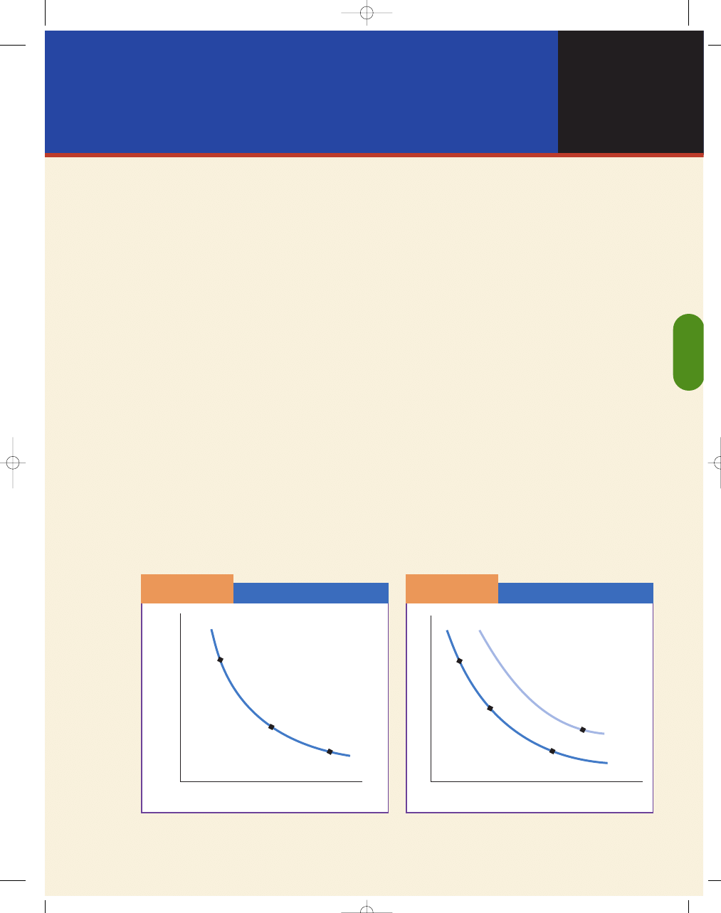
THE PROPERTIES OF THE INDIFFERENCE CURVE

Indifference curves have the following three properties:
(1) Higher indifference curves represent greater satis-
faction, (2) they are negatively sloped, and (3) they
are convex from the origin.

Higher Indifference Curves Represent
Greater Satisfaction

Although consumers are equally happy with any
bundle of goods along the indifference curve, they
prefer to be on the highest indifference curve possible.
This preference follows from the assumption that
more of a good is preferred to less of a good. For
example, in Exhibit 2, the consumer would prefer I

to I

. The higher indifference curve represents more

satisfaction. As you can see in Exhibit 2, bundle D
gives the consumer more of both goods than does
bundle C, which is on a lower indifference curve.
Bundle D is also preferred to bundle A because there
is more than enough extra food to compensate the
consumer for the loss of clothing; total utility has
risen because the consumer is now on a higher indif-
ference curve.

An Indifference Curve

A P P E N D I X

X H I B I T

Indifference

Curve

Quantity of Clothing

Quantity of Food

Indifference Curves

A P P E N D I X

X H I B I T

Quantity of Clothing

Quantity of Food

95469_10_Ch10-p241-270.qxd 29/12/06 12:05 PM Page 261

262

M O D U L E 3

Households, Firms, and Market Structure

Indifference Curves Are Negatively Sloped

Indifference curves must slope downward from left to
right if the consumer views both goods as desirable. If
the quantity of one good is reduced, the quantity of
the other good must be increased to maintain the
same level of total satisfaction.

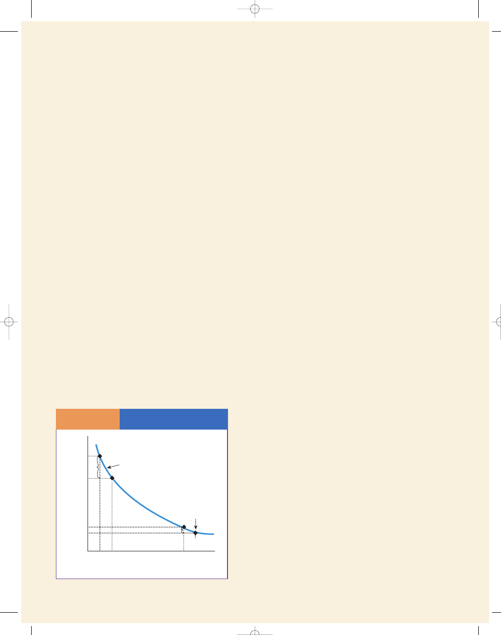
Indifference Curves Are Convex from the Origin

The slope of an indifference curve at a particular
point measures the marginal rate of substitution
(MRS), the rate at which the consumer is willing to
trade one good to gain one more unit of another
good. If the indifference curve is steep, the marginal
rate of substitution is high. The consumer would be
willing to give up a large amount of clothing for a
small amount of food because she would still main-
tain the same level of satisfaction; she would remain
on the same indifference curve, as at point A in
Exhibit 3. If the indifference curve is flatter, the mar-
ginal rate of substitution is low. The consumer is only
willing to give up a small amount of clothing in
exchange for an additional unit of food to remain
indifferent, as seen at point B in Exhibit 3. A con-
sumer’s willingness to substitute one good for another
depends on the relative quantities he consumes. If he
has lots of something, say food relative to clothing, he
will not value the prospect of getting even more food
very highly, which is just the law of demand, which is
based on the law of diminishing marginal utility.

Complements and Substitutes

As we learned in Chapter 4, many goods are comple-
ments to each other; that is, the use of more units of

one encourages the acquisition of additional units of
the other. Gasoline and automobiles, baseballs and
baseball bats, snow skis and bindings, bread and
butter, and coffee and cream are examples of comple-
mentary goods. When goods are complements, units
of one good cannot be acquired without affecting the
want-satisfying power of other goods. Some goods
are substitutes for one another; that is, the more you
have of one, the less you desire the other. (The rela-
tionship between substitutes is thus the opposite of
the relation between complements.) Examples of sub-
stitutes include coffee and tea, sweaters and jackets,
and home-cooked and restaurant meals.

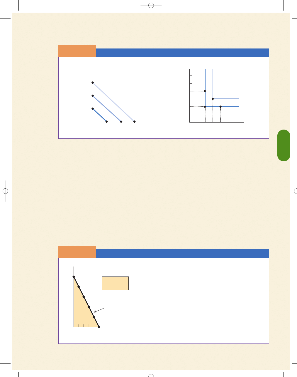
The degree of convexity of an indifference

curve—that is, the extent to which the curve deviates
from a straight line—depends on how easily the two
goods can be substituted for each other. If two com-
modities are perfect substitutes—one $10 bill and two
$5 bills, for example—the indifference curve is a
straight line (in this case, the line’s slope is

−1). As

depicted in Exhibit 4(a), the marginal rate of substi-
tution is the same regardless of the extent to which
one good is replaced by the other.

At the other extreme are two commodities that are

not substitutes but are perfect complements, such as
left and right shoes. For most people, these goods are
never used separately but are consumed only together.
Because it is impossible to replace units of one with
units of the other and maintain satisfaction, the mar-
ginal rate of substitution is undefined; thus, the indif-
ference curve is a right angle, as shown in Exhibit 4(b).
Because most people only care about pairs of shoes, 4
left shoes and 2 right shoes (bundle B) would yield the
same level of satisfaction as 2 left shoes and 2 right
shoes (bundle A). Two pairs of shoes (bundle A) are
also as good as 4 right shoes and 2 left shoes (bundle
C). That is, bundles A, B, and C all lie on the same
indifference curve and yield the same level of satisfac-
tion. But the combination of three right shoes and
three left shoes (bundle D) is preferred to any combi-
nation of bundles on indifference curve I

If two commodities can easily be substituted for

one another, the nearer the indifference curves will
approach a straight line; in other words, it will maintain
more closely the same slope along its length throughout.
The greater the complementarity between the two
goods, the nearer the indifference curves will approach
a right angle.

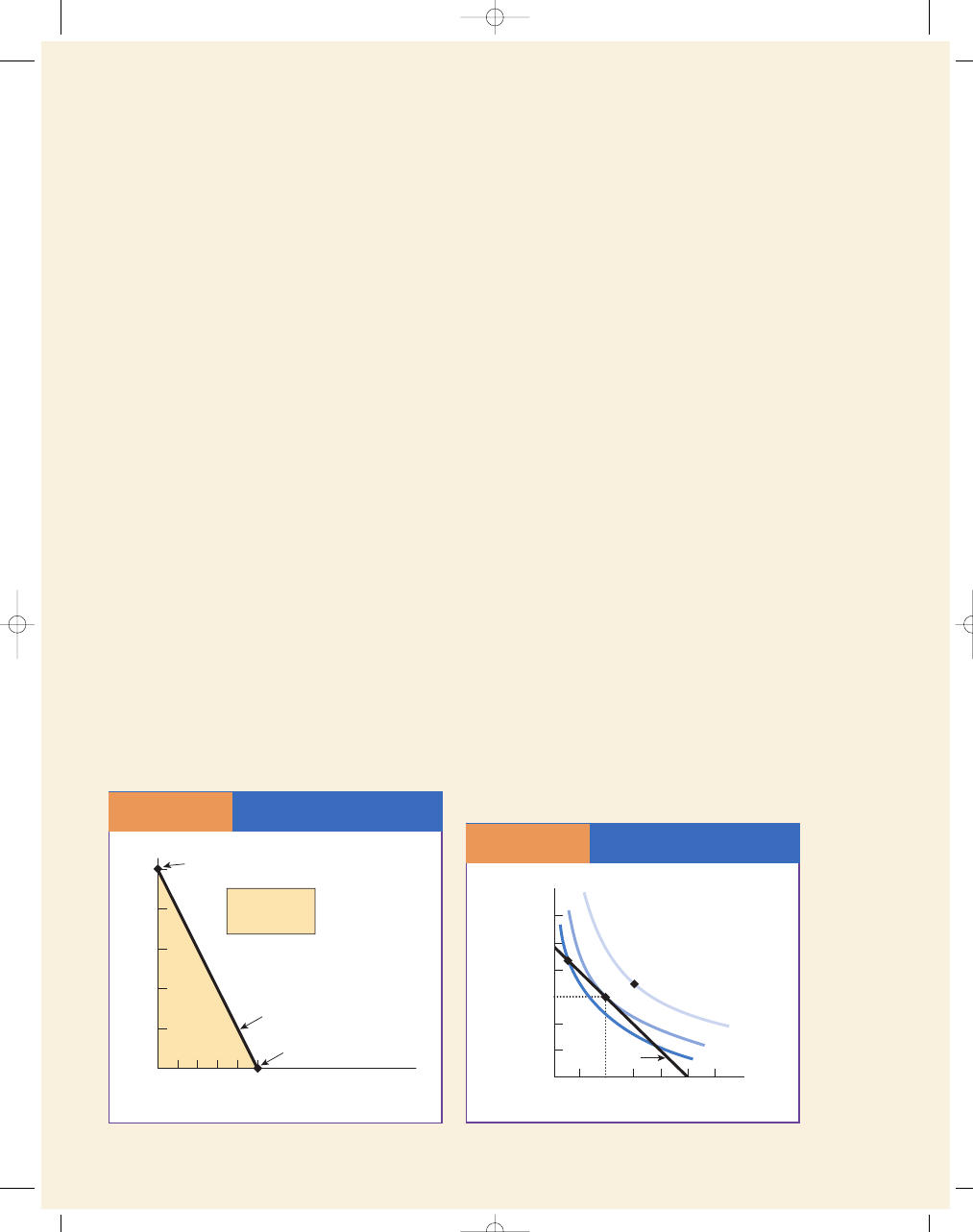
THE BUDGET LINE

A consumer’s purchase opportunities can be illustrated
by a budget line. More precisely, a budget line repre-
sents the various combinations of two goods that a

Indifference Curves Are
Convex from the Origin

A P P E N D I X

X H I B I T

Quantity of Clothing

Quantity of Food

MRS

= 5

MRS

= 1

Indifference

Curve

95469_10_Ch10-p241-270.qxd 29/12/06 12:05 PM Page 262

C H A P T E R 1 0

Consumer Choice Theory

263

consumer can buy with a given income, holding the
prices of the two goods constant. For simplicity, we
only examine the consumer’s choices between two
goods. We recognize that this example is not com-
pletely realistic, as a quick visit to the store shows con-
sumers buying a variety of different goods and services.
However, the two-good model allows us to focus on
the essentials, with a minimum of complication.

First, let’s look at a consumer who has $50 of

income a week to spend on two goods—food and
clothing. The price of food is $10 per unit, and the
price of clothing is $5 per unit. If the consumer
spends all her income on food, she can buy 5 units
of food per week ($50/$10

= 5). If she spends all her

income on clothing, she can buy 10 units of clothing

per week ($50/$5

= 10). However, it is likely that she

will spend some of her income on each. Six of the
affordable combinations are presented in the table in
Exhibit 5. In the graph in Exhibit 5, the horizontal
axis measures the quantity of food and the vertical
axis measures the quantity of clothing. Moving
along the budget line we can see the various combi-
nations of food and clothing the consumer can pur-
chase with her income. For example, at point A, she
could buy 10 units of clothing and 0 units of food;
at point B, 8 units of clothing and 1 unit of food;
and so on.

Of course, any other combination along the budget

line is also affordable. However, any combination of
goods beyond the budget line is not feasible.

Perfect Substitutes and Perfect Complements

A P P E N D I X

X H I B I T

$10 Bills

$5 Bills

Left Shoes

Right Shoes

a. Perfect Substitutes

b. Perfect Complements

The Budget Line

A P P E N D I X

X H I B I T

1 2 3 4

Budget

Line

Not

Affordable

Quantity of Clothing

Quantity of Food

Income

$50

(Food)

$10

(Clothing)

Consumption

Clothing

Food

Total

Opportunities

Clothing

Food

Expenditures

$50

$ 0

$50

95469_10_Ch10-p241-270.qxd 29/12/06 12:05 PM Page 263

264

M O D U L E 3

Households, Firms, and Market Structure

Finding the X- and Y-Intercepts of the Budget Line

The intercept on the vertical Y-axis (the clothing axis)
and the intercept on the horizontal X-axis (the food
axis) can easily be found by dividing the total income
available for expenditures by the price of the good in
question. For example, if the consumer has a fixed
income of $50 a week and clothing costs $5 per unit,
we know that if he spends all his income on clothing,
he can afford 10 (Income/P

= $50/$5 = 10); so 10 is

the intercept on the Y-axis. Now if he spends all his
$50 on food and food costs $10 per unit, he can
afford to buy 5 (Income/P

= $50/$10 = 5); so 5 is the

intercept on the X-axis, as shown in Exhibit 6.

Finding the Slope of the Budget Line

The slope of the budget line is equal to

−P

. The neg-

ative coefficient of the slope indicates that the budget
line is negatively sloped (downward sloping), reflecting
the fact that you must give up some of one good to get
more of the other. For example, if the price of X (food)
is $10 and the price of Y (clothing) is $5, then the slope
is equal to

−10/5, or −2. That is, 2 units of Y can be

obtained by forgoing the purchase of 1 unit of X; hence,
the slope of the budget line is said to be

−2 (or 2, in

absolute value terms) as seen in Exhibit 6.

CONSUMER OPTIMIZATION

So far, we have seen a budget line, which shows the
combinations of two goods that a consumer can afford,
and indifference curves, which represent the con-
sumer’s preferences. Given the consumer’s indifference
curves for two goods, together with the budget line

showing the various quantities of the two that can be
purchased with a given money income for expenditure,
we can determine the optimal (or best) quantities of
each good the consumer can purchase.

The Point of Tangency

The point of tangency between the budget line and an
indifference curve indicates the optimal quantities of
each good that will be purchased to maximize total
satisfaction. At that point of tangency,

−MRS (the

slope of the indifference curve) will be equal to

−P

(the slope of the budget line). Exhibit 7 shows the
consumer’s optimal combination of clothing and
food. The optimum occurs where the budget line is
tangent to indifference curve I

, at point A: The con-

sumer will acquire 2 units of food and 6 units of
clothing.

To maximize satisfaction, the consumer must

acquire the most preferred attainable bundle—that is,
reach the highest indifference curve that can be
reached with a given level of income. The highest
curve that can be reached is the one to which the
budget line is tangent, at point A. Any other possible
combination of the two goods either would be on a
lower indifference curve and thus yield less satisfac-
tion or would be unobtainable with the given income.
For example, point B is affordable but would place
the consumer on a lower indifference curve. In other
words, if the consumer were at point B, she could be
made better off moving to point A by consuming less
clothing and more food. How about point C? That
move would be nice because it is on a higher indiffer-
ence curve and would yield greater total utility, but
unfortunately it is unattainable with the current
budget line.

The Budget Line:
Intercepts and Slopes

A P P E N D I X

X H I B I T

1 2 3

Budget Line

Income

$50

(Food)

$10

(Clothing)

Quantity of Clothing

Quantity of Food

(Income/P

$50/$5 10)

Slope

$10/$5 2

(Income/P

$50/$10 5)

Point of Tangency—The
Consumer’s Optimum

A P P E N D I X

X H I B I T

Budget

Line

Quantity of Clothing

Quantity of Food

95469_10_Ch10-p241-270.qxd 29/12/06 12:05 PM Page 264

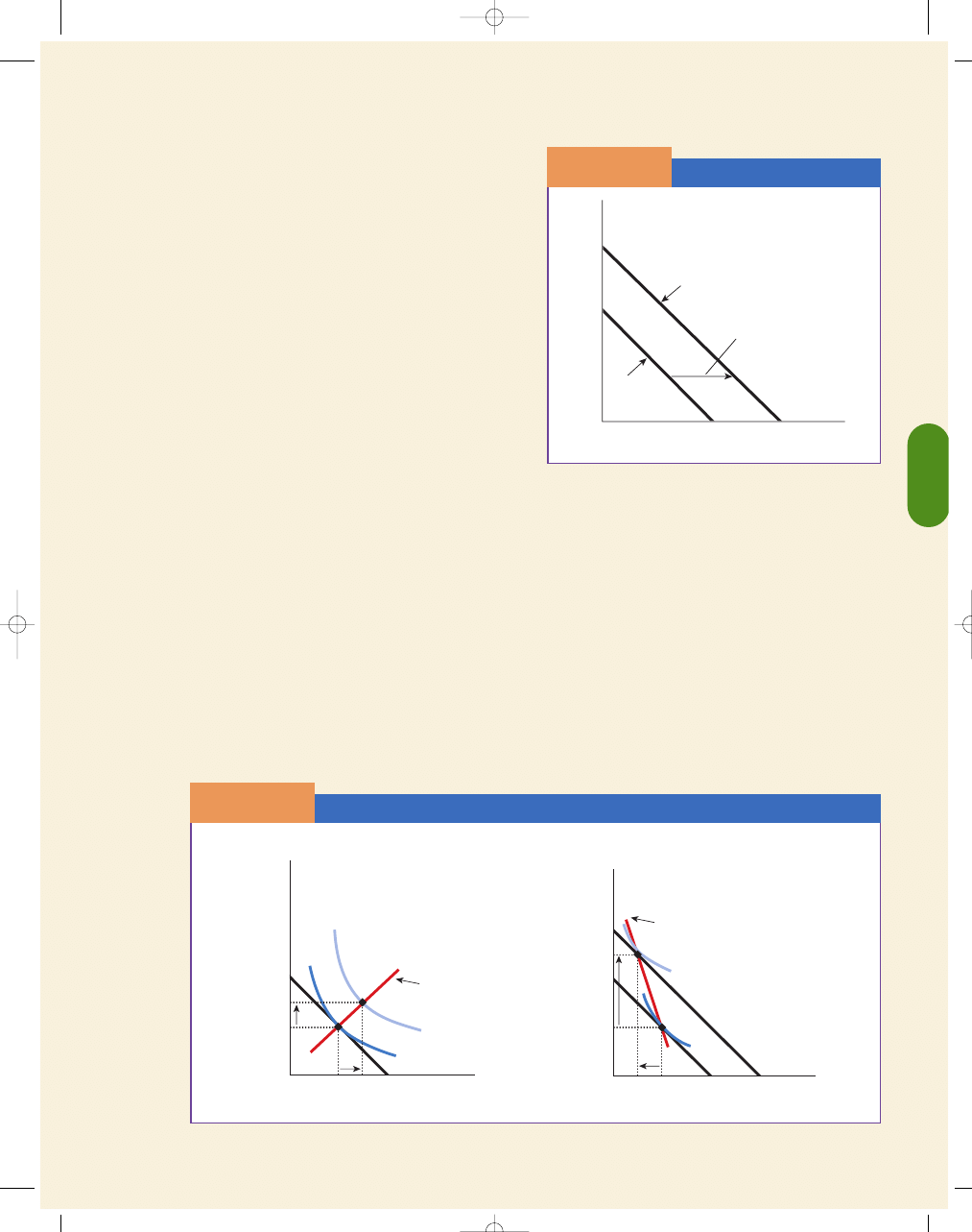
C H A P T E R 1 0

Consumer Choice Theory

265

Change in Income

A P P E N D I X

X H I B I T

Quantity of Clothing

Quantity of Low-Quality Meat

Income
Consumption
Curve

Quantity of Clothing

Quantity of Food

Income
Consumption
Curve

a. Both goods are normal

b. Low-quality meat is the inferior good

CHANGES IN THE BUDGET LINE

So far, we have seen how the prices of goods along
with a consumer’s income determine a budget line.
Now let us examine how the budget line can change
as a result of a change in the income level or the price
of either good.

The Position of the Budget Line If Income Rises

An increase in income, holding relative prices con-
stant, will cause the curve to shift outward, parallel to
the old curve. As seen in Exhibit 8, a richer person can
afford more of both goods than a poorer person
because of the higher budget line. Suppose you just
received an inheritance from a relative; this money
will allow you to now buy more of the things that you
want. The change in income, holding relative prices
constant, is called the income effect and it causes this
parallel shift in the budget line.

With a given pattern of indifference curves, larger

amounts available for spending will result in an
income-consumption curve (ICC) connecting the best
consumption points (tangencies) at each income level.

Consider what happens to consumer purchases

with a rise in income. In Exhibit 9(a), the rise in
income shifts the budget line outward. If both goods,
clothing and food, are normal goods in this range,
then the consumer will buy more of both goods as
seen in Exhibit 9(a). If income rises and the consumer
buys less of one good, we say that good is an inferior
good. In Exhibit 9(b), we see that the consumer buys
more clothing (normal good) but less liver (inferior
good). In this example, as income rises, the consumer
may choose to consume fewer units of liver—the

lower quality meat. Other examples of inferior goods
include secondhand clothing or do-it-yourself hair-
cuts, which consumers generally buy only because
they cannot afford more expensive substitutes.

In Exhibit 9(a), both goods are normal goods, so

the consumer responds to the increase in income by
buying more of both clothing and food. In Exhibit
9(b), clothing is normal and hamburger is an inferior
good, so the consumer responds to the increase in
income by buying more clothing and less hamburger.

The Budget Line Reflects Price Changes

Purchases of goods and services depend on relative
prices as well as a consumer’s level of income.

Change in Income

A P P E N D I X

X H I B I T

An Increase

in Income

Richer

Quantity of Food

Quantity of Clothing

Poorer

95469_10_Ch10-p241-270.qxd 29/12/06 12:05 PM Page 265

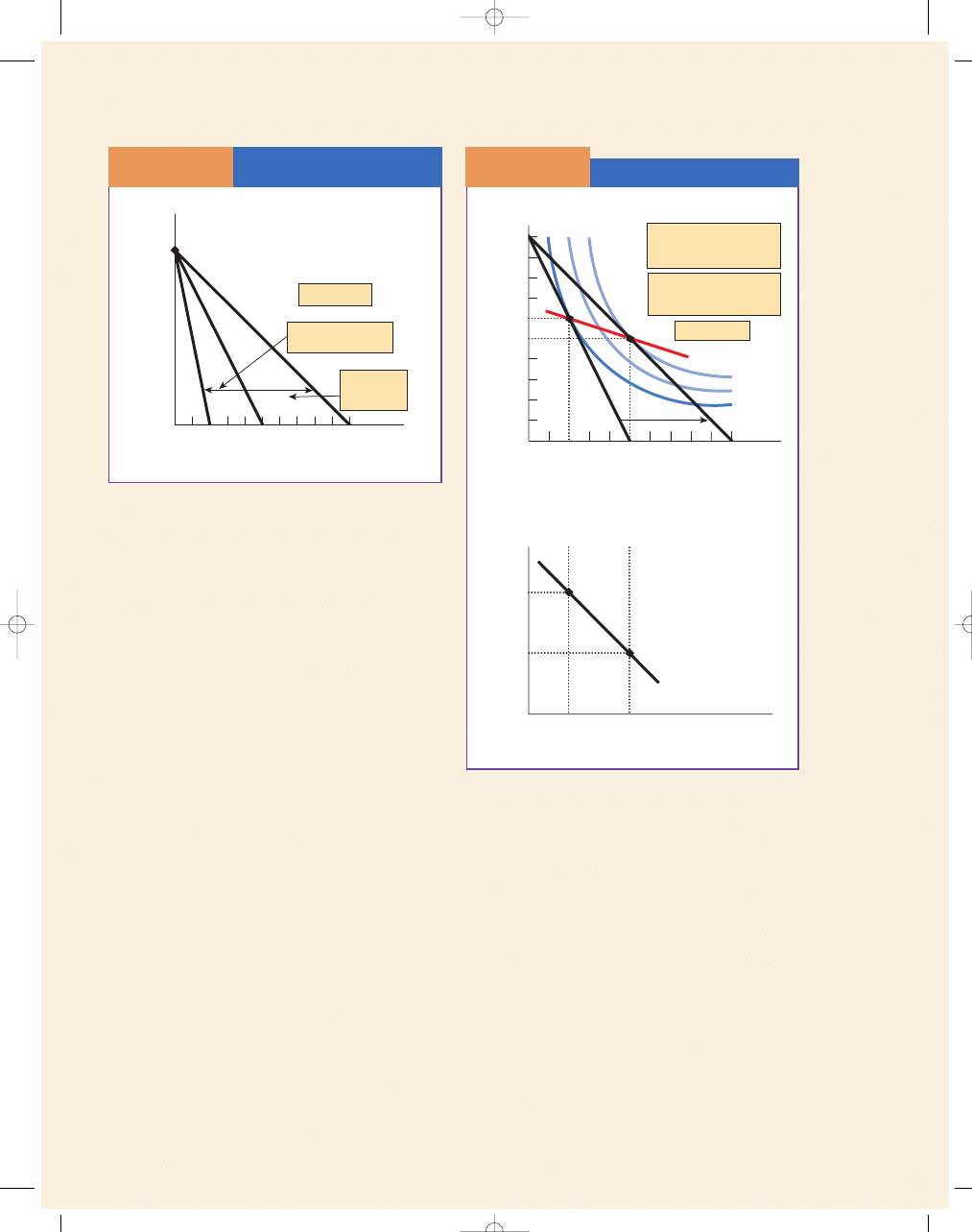
266

M O D U L E 3

Households, Firms, and Market Structure

However, when the price of one good changes, hold-
ing income and the price of the other good constant,
it causes a relative price effect. Relative prices affect
the way consumers allocate their income among dif-
ferent goods. For example, a change in the price of the
good on either the Y- or X-axis will cause the budget
line to rotate inward or outward from the budget
line’s intercept on the other axis.

Let’s return to our two-good example—clothing

and food. Say the price of food falls from $10 to $5.
This decrease in price comes as good news to consumers
because it expands their buying opportunities—rotating
the budget line outward, as seen in Exhibit 10. Thus, a
consumer who spends all his income on food can now
buy 10 units of food, as Income/P

= $50/$5 = 10. If the

price per unit of food rose from $10 to $25, it would
contract the consumer’s buying opportunities and rotate
the budget line inward; so the consumer who spends all
his income on food would be able to buy only 2 units of
food, as Income/P

= $50/$25 = 2.

The tangency relationship between the budget

line and the indifference curve indicates the optimal
amounts of each of the two goods the consumer will
purchase, given the prices of both goods and the con-
sumer’s total available income for expenditures. At
different possible prices for one of the goods, given
the price of the other and given total income, a con-
sumer would optimally purchase different quantities
of the two goods.

A change in the price of one of the goods will

alter the slope of the budget line because a different
amount of the good can be purchased with a given
level of income. If, for example, the price of food falls,
the budget line becomes flatter because the consumer

can purchase more food with a given income than she
previously could. As shown in Exhibit 11, the new
budget line rotates outward, from L

to L

, as a result

of the price reduction. Thus, the new point of tan-
gency with an indifference curve will be on a higher
indifference curve. In Exhibit 11(a), the point of tan-
gency moves from point A to point B as a result of the
decline in price of food from $10 to $5; the equilib-
rium quantity of food purchased increases from 2 to
5 units.

A relation known as the price-consumption curve

(PCC) may be drawn through these points of tan-
gency, indicating the optimum quantities of food (and
clothing) at various possible prices of food (given the
price of clothing). From this price-consumption curve,
we can derive the usual demand curve for the good.
Thus, Exhibit 11(a) shows that if the price of food is
$10, the consumer will purchase 5 units. These data

Change in the Relative
Price of Food

A P P E N D I X

X H I B I T

1 0

1 2 3 4 5

Quantity of Clothing

Quantity of Hamburger

6 7 8 9 10

Income

$50

Price of Food
Falls from
$10 to $5

Price of Food
Rises from $10 to $25

The Price-Consumption Curve

A P P E N D I X

X H I B I T

1 1

Price-
Consumption Curve

Quantity of Clothing

Quantity of Food

9 10

$10

Demand for Food

Price of Food

Quantity of Food

a. Indifference Curve

b. Demand Curve for Food

Budget Line,
Price of $5 for clothing.
$10 for food.

Budget Line,
Price of $5 for clothing.
$5 for food.

Income

$50

95469_10_Ch10-p241-270.qxd 29/12/06 12:05 PM Page 266

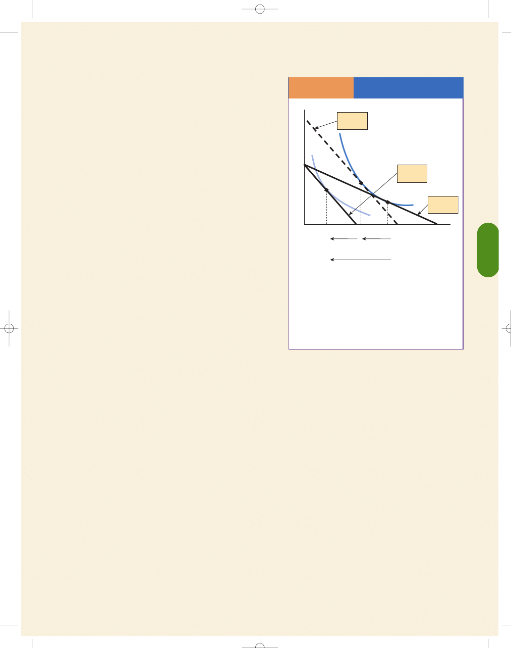
C H A P T E R 1 0

Consumer Choice Theory

267

may be plotted, as in Exhibit 11(b), to derive a demand
curve of the usual form. Notice that in Exhibit 11(b)
the price of food is measured on the vertical axis and the
quantity purchased on the horizontal axis, whereas the
axes of Exhibit 11(a) refer to quantities of the two
goods. Notice also that the quantities demanded, as
shown in Exhibit 11(b), are those with the consumer’s
expenditures in equilibrium (at her optimum) at the
various prices. Essentially, the demand curve is made
up of various price and quantity optimum points.

THE INCOME AND SUBSTITUTION EFFECTS
OF A PRICE CHANGE

With indifference curves, we can easily see the two
ways in which a price reduction influences the quan-
tity demanded. When the price of a good falls, the
income effect enables the person to buy more of this
good (or other goods) with a given income; the price
reduction has the same effect as an increase in money
income. That is, the consumer can now move onto a
higher indifference curve.

The second influence of the price decline on the

quantity demanded is the substitution effect. The
lower price encourages the consumer to buy larger
quantities of this good. The substitution effect is
always negative. That is, price and quantity demanded
are negatively correlated; lower prices mean higher
quantities demanded, and vice versa.

Exhibit 12 shows the income and substitution

effects for an increase in the price of pizza. Because
the relative price of pizza increases, the budget line
rotates inward. (Note that the Y-intercept did not
change, because neither income nor the price of pizza
changed. Hence if all income is spent on Coke before
and after the price increase of pizza, the same amount
of Coke can be purchased). The total effect of the
increase in the price of pizza is indicated by point c,
that is; a reduction in the quantity of pizza from 7
slices of pizza to 3 slices of pizza.

Within the total effect are the substitution effect

and the income effect. First consider how much of the
total effect is substituting away from the now higher-
priced good, pizza. This comparison can easily be
made by taking the new budget line and drawing a
new hypothetical budget line parallel to the new
budget line but tangent to the old indifference curve
I

. Why? It shows the effect of the new relative price

on the old indifference curve—in effect, the consumer
is compensated for the loss of welfare associated with
the price rise by enough income to return to the orig-
inal indifference curve, I

. Remember that as long as

the new budget line and the hypothetical budget line
are parallel, the relative prices are the same; the only

difference is the level of income. Thus, we are able to
isolate the one effect—the amount of substitution that
would prevail without the real income effect—which is
the movement from a to b, or the substitution effect.

The movement from b to c is a change in the real

income when the relative prices are constant, because
this move requires a parallel shift in the budget line.
Thus, the movement from b to c results from the
decrease in real income because of the higher price of
pizza while all other prices remain constant—the
income effect. Remember that the slope of the budget
line indicates relative prices; thus, by shifting the new
budget line next to the old indifference curve, we can
see the change that took place holding real income
(measured by utility) constant. Then when we make
the parallel shift, we see that the change in income,
because the size of the parallel shift measures only
the amount of real income change, with relative prices
remaining constant.

SUBSIDIES AND INDIFFERENCE CURVES

The indifference curve is a convenient tool to aid in
our understanding of subsidies. In this final section,
we will consider two examples demonstrating the

The Income and Substitution
Effects

A P P E N D I X

X H I B I T

1 2

Quantity of Coke (per week)

Quantity of Pizza (slices per week)

Income

effect

Total effect

Substitution

effect

Hypothetical

Budget Line

Initial

Budget Line

New

Budget Line

An increase in the price of pizza causes an inward rota-
tion of the budget line. The substitution effect, a to b,
is measured along the original indifference curve. The
income effect is measured by a parallel shift of the
budget lines from the hypothetical budget line to the
new budget line.

95469_10_Ch10-p241-270.qxd 29/12/06 12:05 PM Page 267

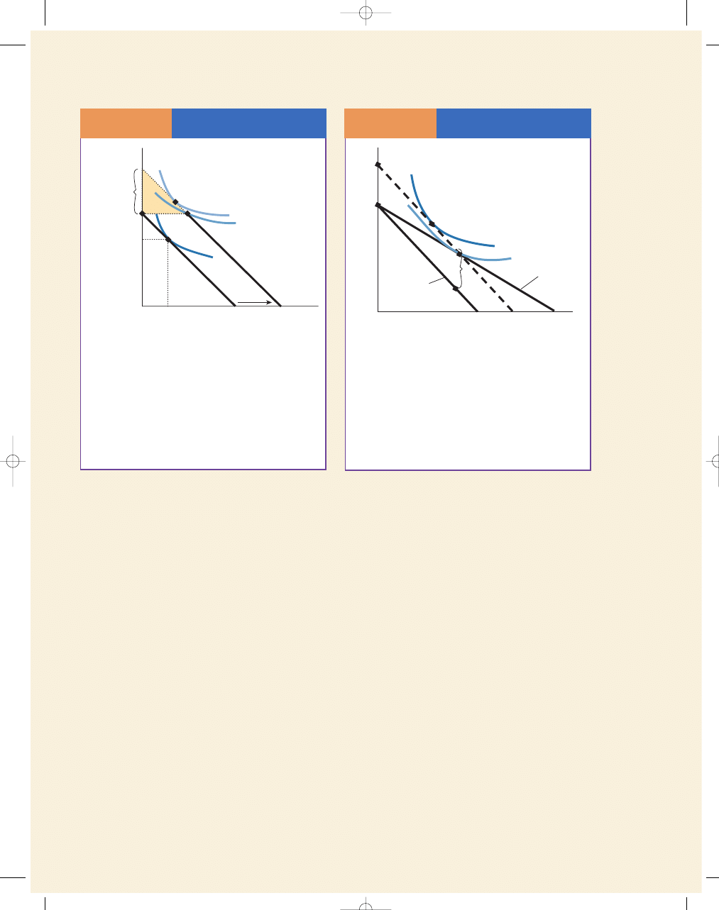
268

M O D U L E 3

Households, Firms, and Market Structure

effects of subsidies in income as compared to subsidies
in price. The first question is whether the poor would
be better off with cash or food stamps. The second
example has to do with the more general question of
subsidizing the price of a good like buses or trains.

Using the indifference curve approach, we can

show that the poor would be at least equally as well off
receiving cash rather than a subsidy like food stamps.

In Exhibit 13, if the individual’s initial position is

at a (consuming F

amount of food, an amount deemed

insufficient by society), the introduction of a food
stamp program that allowed the recipient to spend an
additional $100 per month exclusively on food would
make the consumer better off (bundles of indifference
curve I

are preferred to those on I

). However, for the

same expense, this individual might be made even
better off by receiving $100 in cash. The reason is that
the shaded triangle is unobtainable to the recipient of
food stamps but not to those receiving a cash payment.
Unless the individual intended to spend all of the next
$100 of additional income on food, he or she would be
better off with a choice.

Similarly, subsidizing the price of a good (like

education, postal services, mass transportation, or
medical services) is usually not the best method to

assure that society’s scarce resources are properly
allocated. If the price of a good is subsidized, it dis-
torts market signals and results in output levels of the
subsidized good that are inefficiently large. In other
words, the opportunity cost of forgone other goods
that could have been produced with those resources is
greater than the (marginal) value of the subsidized
good. (Recall the ordinary supply and demand dia-
gram for a subsidy from your elementary economics
course.) Exhibit 14 shows that if the whole budget
constraint is shifted parallel by an amount equivalent
to the price subsidy, ab (ab

= cd), then a higher indif-

ference curve can be reached. Because reaching the
highest indifference curve subject to the budget con-
straint maximizes consumer satisfaction, this simple
diagram shows that it is better to subsidize income
(parallel shift) than to subsidize price (altering the
slope), if one is interested in making some group
better off. Of course, if you want certain groups (say,
the poor) to consume more of particular goods (hous-
ing or food), rather than just raising their utility you
may not wish to give unconstrained income subsidies.
Recall that economists can never, in their role as econo-
mists, recommend one approach over the other but they
can point out the implications of alternative choices.

Cash Grants Versus Food
Stamp Income Subsidy

A P P E N D I X

X H I B I T

1 3

$100

AOG

Quantity of All

Other Goods (A

OG)

Quantity of Food

(monthly)

(Cash)

(Food stamps)

With no government assistance, the consumer chooses
bundle a. The availability of food stamps increases the
budget and allows the buyer to purchase bundle b, con-
suming more food and more other goods and attaining
a higher level of utility. A cash grant, however, expands
the budget set further. The recipient would purchase
bundle c, which contains more nonfood items and less
food than bundle b. The consumer reaches a higher
level of utility with a cash grant than with food stamps.

Cash Grants Versus Price
Subsidies

A P P E N D I X

X H I B I T

1 4

Quantity of All

Other Goods (A

OG)

Subsidized Good

(buses, postal services, Amtrak)

Apparent

(subsidized)

Cost Trade-Off

True Cost
Trade-Off

A subsidy lowers the price paid for the good,
pivoting the budget line to the right, whereas a
cash grant causes a parallel shift of the budget line
to the right. The consumer chooses bundle a with
the subsidy but attains more satisfaction under a
cash grant program. More units of the subsidized
good and fewer units of other goods are consumed
with a subsidy than with a cash grant of equivalent
value.

95469_10_Ch10-p241-270.qxd 29/12/06 12:05 PM Page 268

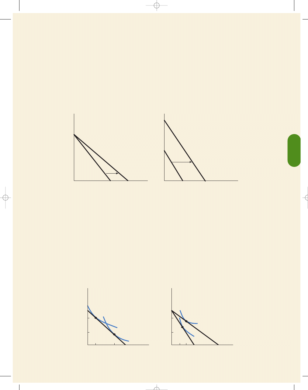
C H A P T E R 1 0

Consumer Choice Theory

269

Problems

1. If you had a budget of $200, and the P

is $5 and the P

is $10, draw the budget line. Draw the budget lines when

the P

falls to $8. Show the budget line when the money available for expenditures increases to $400. What is the

slope of the budget line when P

is $5 and P

is $10? How about when P

falls to $8?

Answer

The intercepts in part (a) are E/P

, $200/$5

= 40 and E/P

or $200/$10

= 20. When P

falls to $8, the budget line

rotates outward from L

to L

; and now E/P

is $200/$8 or 25. In part (b), the intercepts are E/P

, or $400/$5

= 80,

and E/P

or $400/10

= 40. Part (b) shows that budget line L

is parallel to L

. The slope of this budget line is

−P

= −$10/$5 or −2. The slope of the budget line when P

falls to $8 is

−8/5, or −1.6.

2. Joe buys more clothes than Jim.

a. Using indifference curves, show how Jim’s consumption of clothing and food may differ from Joe’s because they

have different tastes, ceteris paribus.

b. Suppose that Jim and Joe have the same tastes and income. Joe’s father manages a clothing store, and Joe is able to

buy all his clothes at wholesale prices. Show why Jim’s choices of food and clothing differ from Joe’s in this situation.

c. Now suppose that Jim and Joe have the same tastes and face the same prices, but that Joe has more money to spend

than Jim. Demonstrate how this difference affects Joe’s consumption pattern compared with Jim’s.

Answer

Part (a) shows that Joe and Jim have different indifference curves because Joe’s preferences are biased toward clothing and
thus Joe purchases more clothing than Jim. Note that because the indifference curves are from separate preference maps,
they can intersect. In part (b), Joe can buy clothes at a reduced price, so his budget line rotates outward from Jim’s and he
buys more clothes. Joe has more income than Jim in part (c), so Joe’s budget line is positioned to the right of Jim’s.

Food

Jim

Food

Joe

Jim

Joe

Food per

Clothing per Year

a. Joe has greater preferences
for clothing

b. Joe faces lower clothing prices
than Jim

Food

Joe

Food

Jim

Joe

Jim

Joe

Jim

Food per

Clothing per Year

95469_10_Ch10-p241-270.qxd 29/12/06 12:05 PM Page 269

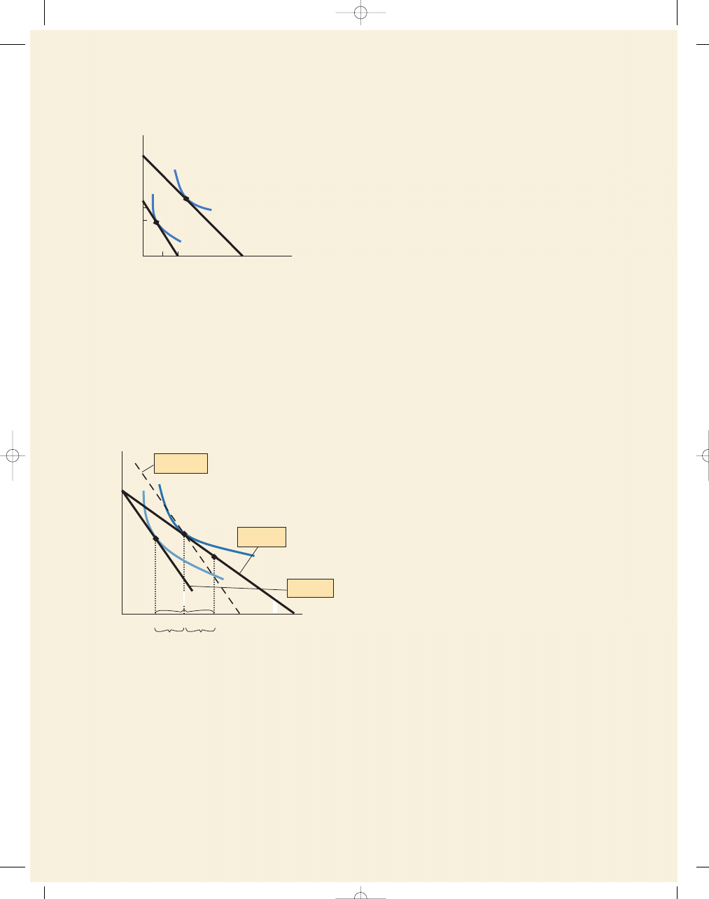
270

M O D U L E 3

Households, Firms, and Market Structure

3. Cigarette taxes are imposed to discourage consumption of so-called “undesirable goods.” Using indifference curves,

show the effect of an increase in taxes on cigarettes. What is the total effect? How much of the change is due to the
income effect? How much is due to the substitution effect?

Answer

The desired effect is to reduce consumption of cigarettes by increasing its relative price. The total effect of the reduc-
tion in consumption is 7 to 3 packs of cigarettes per week. The distance between point a to a

′ represents the reduc-

tion due to the substitution effect. That is, substitution occurs which favors other goods relative to the now more
expensive cigarettes. The other component of the total effect is the income effect. The income effect shows the loss in
real income due to the price increase—a movement from a

′ to b.

Quantity of All Other Goods

Quantity of Cigarettes

(packs per month)

′

Hypothetical

Budget Line

New

Budget Line

Initial

Budget Line

Income Effect

(3–5)

AOG

Substitution Effect

(5–7)

Total Effect

(3–7)

c. Joe has more money available
for expenditures

Food

Joe

Food

Jim

Joe

Jim

Joe

Jim

Food per

ear

Clothing per Year

95469_10_Ch10-p241-270.qxd 29/12/06 12:05 PM Page 270