Exploring Economics 4e Chapter 26

C H A P T E R

26.1

Simple Keynesian Expenditure Model

26.2

Finding Equilibrium in the Keynesian Model

26.3

Adding Investment, Government Purchases,
and Net Exports

26.4

Shifts in Aggregate Expenditure and the
Multiplier

26.5

A Complete Model

26.6 Government Purchases, Taxes, and the

Balanced-Budget Multiplier

26.7

The Paradox of Thrift

26.8

Keynesian-Cross to Aggregate Demand

H E

E Y N E S I A N

X P E N D I T U R E

O D E L

H E

E Y N E S I A N

X P E N D I T U R E

O D E L

he Keynesian expenditure model is based on
the condition that the components of aggre-
gate demand (consumption, investment, gov-
ernment purchases, and net exports) must equal

total output. Keynes believed that total spending
was the critical determinant of the overall level

of economic activity. When total spending
increases, firms increase their output and hire
more workers. Even though Keynes ignored an
important component—aggregate supply—his
model still provides a great deal of information
about aggregate demand.

■

95469_26_Ch26_p719-752.qxd 14/1/07 3:00 PM Page 719

WHY DO WE ASSUME THE PRICE LEVEL IS FIXED?

In most of this chapter, we will assume that the price
level is fixed or constant. If the price level is fixed,
then changes in nominal income will be equivalent to
changes in real income. That is, when we assume the
price level is fixed, we do not have to distinguish real
variable changes from nominal variable changes.
Keynes believed that prices and wages were rigid or
fixed until we reached full employment. But let us
begin by looking at the most important aggregate
demand determinant—consumption.

THE SIMPLEST KEYNESIAN EXPENDITURE MODEL:
AUTONOMOUS CONSUMPTION ONLY

It is useful to begin by considering consumption spending
by households. Household spending on goods and serv-
ices is the largest single component of the demand for
final goods, accounting for more than 65 percent of GDP.

Numerous economic variables influence aggre-

gate demand for consumer goods and services, and
thus, aggregate consumption expenditures. Using you
or your family as an example, you know that such
things as family disposable income (after-tax income),
credit conditions, the level of debt outstanding, the
amount of financial assets, and expectations are impor-
tant determinants of consumption purchases. Most
economists believe that disposable income is one of the
dominant factors.

Let’s begin by simplifying things quite a bit. Imagine

an economy in which only consumption spending exists
(no investment, government purchases, or net exports;
later, we’ll add in these other sectors). To begin with the
simplest situation possible, let’s suppose that each house-
hold has the same level of disposable income. This kind
of analysis that relies on averages is called a representa-
tive household analysis. On a graph of consumption
spending (vertical axis) for our representative household
and the household’s representative disposable income
(horizontal axis), we could represent average consump-
tion of disposable income at point A in Exhibit 1. From
point A, a horizontal dotted line to the vertical axis
permits us to read the value of average consumption
spending, C

WHAT ARE THE AUTONOMOUS FACTORS
THAT INFLUENCE SPENDING?

Even though income is given for the representative
household, other economic factors that influence con-
sumption spending are not. When consumption (or
any of the other components of spending, such as
investment) does not depend on income, we call it
autonomous (or independent). Let’s look at some of
these other autonomous factors and see how they
would change consumption spending.

Real Wealth

The larger the value of a household’s real wealth (the
money value of wealth divided by the price level,
which indicates the amount of consumption goods

720

M O D U L E 6

Macroeconomic Foundations

S E C T I O N

26.1

S i m p l e K e y n e s i a n E x p e n d i t u r e M o d e l

■

Why do we assume a fixed price level?

■

What economic variables influence aggregate
demand?

■

What are the autonomous factors that
influence consumption spending?

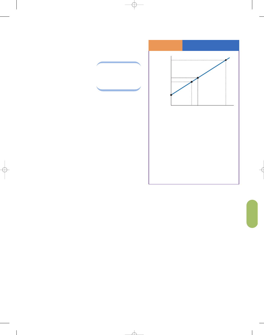
Autonomous Changes in
Consumption Spending

S E C T I O N

2 6 .1

X H I B I T

An increase in real wealth would raise consumption
spending to C

, at point D. A decrease in real wealth

would tend to lower the level of consumption
spending to C

, at point B. A higher interest rate tends

to cause a decrease in consumption spending from
point A to point B. As household debt increases, other
things equal, consumption spending would fall from
point A to point B. In general, an increase in consumer
confidence would act to increase household spending
(a movement from point A to point D) and a decrease
in consumer confidence would act to decrease house-
hold spending (a movement from point A to point B).

Disposable Income (DY )

Representative Household

Consumption Expenditures

95469_26_Ch26_p719-752.qxd 14/1/07 3:00 PM Page 720

C H A P T E R 2 6

The Keynesian Expenditure Model

721

that the wealth could buy), the larger the amount of
consumption spending, other things equal. Thus, in
Exhibit 1, an increase in real wealth would raise con-
sumption to C

, at point D, for a given level of current

income. Similarly, something that would lower the
value of real wealth, such as a decline in property
values or a stock market decline would tend to lower
the level of consumption to C

, at point B in Exhibit 1.

The Interest Rate

A higher interest rate tends to make the consumption
items that we buy on credit more expensive, which
reduces expenditures on those items. An increase in the
interest rate increases the monthly payments made to
buy such things as automobiles, furniture, and major
appliances and reduces our ability to spend out of a given
income. This shift is shown as a decrease in consumption
from point A to point B in Exhibit 1. Moreover, an
increase in the interest rate provides a higher future
return from reducing current spending, which motivates
increasing savings. Thus, a higher interest rate in the cur-
rent period would likely motivate an increase in savings
today, which would permit households to consume more
goods and services at some future date.

Household Debt

Remember when that friend of yours ran up his credit
card obligations so high that he stopped buying goods
except the basic necessities? Well, our average house-
hold might find itself in the same situation if its out-
standing debt exceeds some reasonable level relative
to its income. So, as debt increases, other things equal,
consumption expenditure would fall from point A to
point B in Exhibit 1.

Expectations

Just as in microeconomics, decisions to spend may
be influenced by a person’s expectations of future

disposable income, employment, or certain world events.
Based on monthly surveys conducted that attempt
to measure consumer confidence, an increase in con-
sumer confidence generally acts to increase household
spending (a movement from point A to point D in
Exhibit 1) and a decrease in consumer confidence
would act to decrease spending (a movement from A
to B in Exhibit 1). For example, a decline in the con-
sumer confidence index after the Iraqi invasion of
Kuwait and a subsequent fall in household spending
are considered factors in the 1990–1991 recession in
the United States.

Tastes and Preferences

Of course, each household is different. Some are young
and beginning a working career; some are without chil-
dren; others have families; still others are older and per-
haps retired from the workforce. Some households like
to save, putting dollars away for later spending, while
others spend all their income, or even borrow to
spend more than their current disposable income.
These saving and spending decisions often vary over a
household’s life cycle.

As you can see, many economic factors affect

consumption expenditures. The factors already listed
represent some of the most important. All of these
factors are considered

autonomous determinants of

consumption expen-
ditures;

that is, those

expenditures that are
not dependent on the
level of current dispos-
able income. Now let’s
make our model more
complete and evaluate
how changes in dis-
posable income affect
household consumption
expenditures.

S E C T I O N

C H E C K

The Keynesian expenditure model is based on the idea that the components of aggregate demand must equal total

output, implying that changes in aggregate demand cause fluctuations in real GDP.

In the simplest model, the price level is fixed to allow for easy evaluation of changes in demand due to real income.

In the simplest model, consumption spending is the primary determinant of aggregate demand.

Representative household analysis allows the determination of the value of average consumption spending.

Autonomous consumption is not dependent on income and includes real wealth, the interest rate, household debt,

future expectations, and tastes and preferences.

autonomous deter-
minants of consump-
tion expenditures

expenditures not dependent on the
level of current disposable income
that can result from factors such as
real wealth, the interest rate, house-
hold debt, expectations, and tastes
and preferences

95469_26_Ch26_p719-752.qxd 14/1/07 3:00 PM Page 721

722

M O D U L E 6

Macroeconomic Foundations

In our first model, we looked at the economic variables
that affected consumption expenditures when dispos-
able income was fixed. This assumption is clearly unre-
alistic, but it allows us to develop some of the basic
building blocks of the Keynesian expenditure model.
Now we’ll look at a slightly more complicated model in
which consumption also depends on disposable income.

If you think about what determines your own

current consumption spending, you know that it
depends on many factors previously discussed, such
as your age, family size, interest rates, expected
future disposable income, wealth, and, most impor-
tantly, your current disposable income. Recall from
earlier chapters, disposable income is your after-tax
income. Your personal consumption spending
depends primarily on your current disposable
income. In fact, empirical studies confirm that most
people’s consumption spending is closely tied to their
disposable income.

REVISITING MARGINAL PROPENSITY
TO CONSUME AND SAVE

What happens to current consumption spending when
a person earns some additional disposable income?
Most people will spend some of their extra income

and save some of it.
The percentage of your
extra disposable income
that you decide to spend
on consumption is what
economists call your

marginal propensity
to consume (MPC).

That is, MPC is equal to the change in consumption
spending (

∆C) divided by the change in disposable

income (

∆DY).

MPC

= ∆C/∆DY

For example, suppose you won a lottery prize of
$1,000. You might decide to spend $750 of your win-
nings today and save $250. In this example, your
marginal propensity to consume is 0.75 (or 75%)
because out of the extra $1,000, you decided to spend
75 percent of it (0.75

× $1,000 = $750).

The term marginal propensity to consume has

two parts: (1) marginal refers to the fact that you
received an extra amount of disposable income—in
addition to your income, not your total income; and
(2) propensity to consume refers to how much you
tend to spend on consumer goods and services out of
your additional income.

How does the assumption of a fixed price level in the Keynesian expenditure model solve the problem of distin-

guishing between changes in the real value of a variable (such as GDP) and changes in its nominal value?

Would it be possible for some consumption expenditures to be autonomous and other parts of consumption

expenditures not to be autonomous?

In what two ways does a higher interest rate tend to reduce current consumption?

What would happen to autonomous consumption expenditures if the value of a consumer’s stock market invest-

ments rose and his household debt rose at the same time?

What would happen to your autonomous consumption if you expected to get a job paying 10 times your current

salary next week?

Why do households headed by a 50-year-old tend to save a larger fraction of their incomes than those headed by

either a 30-year-old or a 70-year-old?

S E C T I O N

26.2

F i n d i n g E q u i l i b r i u m i n t h e K e y n e s i a n M o d e l

■

What factors determine consumer spending?

■

How do we find equilibrium in the Keynesian
model?

■

Why does income equal output?

■

Why does expenditure equal output?

marginal propensity
to consume (MPC)

the additional consumption that
results from an additional dollar
of income

95469_26_Ch26_p719-752.qxd 14/1/07 3:00 PM Page 722

C H A P T E R 2 6

The Keynesian Expenditure Model

723

MARGINAL PROPENSITY TO SAVE

The flip side of the marginal propensity to consume is
the

marginal propensity to save (MPS),

which is the

proportion of an addi-
tion to your income
that you would save or
not spend on goods and
services today. That is,
MPS is equal to the
change in savings (

∆S)

divided by the change in
disposable income (

∆DY).

MPS

= ∆S/∆DY

In the earlier lottery example, your marginal

propensity to save is 0.25, or 25 percent, because you
decided to save 25 percent of your additional disposable
income (0.25

× $1,000 = $250). Because your additional

disposable income must be either consumed or saved,
the marginal propensity to consume plus the marginal
propensity to save must add up to 1, or 100 percent.

Let’s illustrate the marginal propensity to consume

in Exhibit 1. Suppose you estimated that you had to
spend $8,000 a year, even if you earned no income for
the year, for “necessities” such as food, clothing, and
shelter. And suppose for every $1,000 of added dis-
posable income you earn, you spend 75 percent of it
and save 25 percent of it. So if your disposable income
is $0, you spend $8,000 (that means you have to
borrow or reduce your existing savings just to survive).
If your disposable income is $20,000, you’ll spend
$8,000 plus 75 percent of $20,000 (which equals
$15,000), for total spending of $23,000. If your dis-
posable income is $40,000, you’ll spend $8,000 plus
75 percent of $40,000 (which equals $30,000), for
total spending of $38,000.

What’s your marginal propensity to consume? In

this case, if you spend 75 percent of every additional
$1,000 you earn, your marginal propensity to con-
sume is 0.75 or 75 percent. And if you save 25 percent
of every additional $1,000 you earn, your marginal
propensity to save is 0.25.

In Exhibit 1, the slope of the line represents the mar-

ginal propensity to consume. To better understand this
concept, look at what happens when your disposable
income rises from $18,000 to $20,000. At a disposable
income of $18,000, you spend $8,000 plus 75 percent of
$18,000 (which is $13,500), for total spending of
$21,500. If your disposable income rises to $20,000,
you spend $8,000 plus 75 percent of $20,000 (which
is $15,000), for total spending of $23,000. So when
your disposable income rises by $2,000 (from $18,000

to $20,000), your spending goes up by $1,500 (from
$21,500 to $23,000). Your marginal propensity to
consume is $1,500 (the increase in spending) divided
by $2,000 (the increase in disposable income), which
equals 0.75, or 75 percent. But notice that this calcu-
lation is also the calculation of the slope of the line
from point A to point B in the exhibit. Recall that the
slope of the line is the rise (the change on the vertical
axis) over the run (the change on the horizontal axis).
In this case, that’s $1,500 divided by $2,000, which
makes 0.75 the marginal propensity to consume. So
the marginal propensity to consume is the same as the
slope of the line in our graph of consumption and dis-
posable income.

Now, let’s take this same logic and apply it to the

economy as a whole. If we add up, or aggregate,
everyone’s consumption and everyone’s income, we’ll get
a line that looks like the one in Exhibit 1, but that applies
to the entire economy. This line or functional relation-
ship is called a consumption function. Let’s suppose
consumption spending in the economy is $1 trillion plus
75 percent of income.

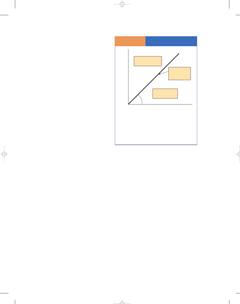
The Marginal Propensity
to Consume

S E C T I O N

2 6 . 2

X H I B I T

The slope of the line represents the marginal
propensity to consume. At a disposable income
of $18,000, you spend $8,000 plus 75 percent of
$18,000 (which is $13,500), for total spending of
$21,500. If your disposable income rises to $20,000,
you spend $8,000 plus 75 percent of $20,000
(which is $15,000), for total spending of $23,000.
So when your disposable income rises by $2,000
(from $18,000 to $20,000), your spending goes up
by $1,500 (from $21,500 to $23,000). Your marginal
propensity to consume is $1,500 (the increase in
spending) divided by $2,000 (the increase in dispos-
able income), which equals 0.75, or 75 percent. But
notice that this MPC calculation is also the calculation
of the slope of the line from point A to point B.

marginal propensity
to save (MPS)

the additional saving that results
from an additional dollar of income

Disposable Income

Consumption Function

$8,000

$18,000

$20,000

$40,000

$21,500

$23,000

$38,000

Consumption Expenditures

95469_26_Ch26_p719-752.qxd 14/1/07 3:00 PM Page 723

724

M O D U L E 6

Macroeconomic Foundations

Now, with consumption equal to $1 trillion plus

75 percent of income, consumption is partly auto-
nomous (the $1 trillion part, which people would
spend no matter what their income, which depends
on the current interest rate, real wealth, debt, and
expectations), and partly induced, which means it
depends on income. The induced consumption is the
portion that’s equal to 75 percent of income.

What is the total amount of expenditure in this

economy? Because we’ve assumed that investment, gov-
ernment purchases, and net exports are zero, aggregate
expenditure is just equal to the amount of consumption
spending represented by our consumption function.

EQUILIBRIUM IN THE KEYNESIAN MODEL

The next part of the Keynesian expenditure model is to
examine what conditions are needed for the economy to
be in equilibrium. This discussion also tells us why the
Keynesian expenditure model is sometimes called a
Keynesian-cross model. In order to determine equilib-
rium, we need to show (1) that income equals output in
the economy, and (2) that in equilibrium, aggregate
expenditure (or consumption in this example) equals
output. First, income equals output because people earn
income by producing goods and services. For example,
workers earn wages because they produce some product
that is then sold on the market, and owners of firms
earn profits because the products they sell provide more
income than the cost of producing them. So any income
that is earned by anyone in the economy arises from the
production of output in the economy. From now on,
we’ll use this idea and say that income equals output;
we’ll use the terms income and output interchangeably.
Another way to remember this concept is to refer to the
circular flow diagram (see Exhibit 1 in Section 22.1 on
page 605). The top half (output) is always equal to the
bottom half (income—the sum of wages, rents, interest
payments, and profits).

The second condition needed for equilibrium

(aggregate expenditure in the economy equals output)
is the distinctive feature of the Keynesian expenditure
model. Just as income must equal output (because
income comes from selling goods and services), aggre-
gate expenditure equals output because people can’t
earn income until the products they produce are sold
to someone. Every good or service that is produced in
the economy must be purchased by someone or added
to inventories. Exhibit 2 plots aggregate expenditure
against output. As you can see, it’s a 45-degree line
(slope

= 1). The 45-degree line shows that the number

on the horizontal axis, representing the amount of
output in the economy, real GDP (Y ), is equal to the
number on the vertical axis, representing the amount

of real aggregate expenditure (AE ) in the economy. If
output is $5 trillion, then in equilibrium, aggregate
expenditure must equal $5 trillion. All points of
macroeconomic equilibrium lie on the 45-degree line.

EQUILIBRIUM IN THE KEYNESIAN MODEL

What would happen if, for some reason, output were
lower than its equilibrium level, as would be the case
if output were Y

in Exhibit 3?

Looking at the vertical dotted line, we see that

when output is Y

, aggregate expenditure (shown by the

consumption function) is greater than output (shown by
the 45-degree line). This amount is labeled the distance
AB on the graph. So people would be trying to buy more
goods and services (A) than were being produced (B),
which would cause producers to increase the amount of
production, which would increase output in the econ-
omy. This process would continue until output reached
its equilibrium level, where the two lines intersect.
Another way to think about this disequilibrium is that
consumers would be buying more than is currently pro-
duced, causing a decrease in inventories on shelves and
in warehouses from their desired levels. Clearly, profit-
seeking businesspeople would increase production to
bring their inventory stocks back up to the desired
levels. In doing so, they would move production to the
equilibrium level.

In Equilibrium, Aggregate
Expenditure Equals Output

S E C T I O N

2 6 . 2

X H I B I T

The 45-degree line shows that the number on the hor-
izontal axis, representing the amount of output in the
economy, is equal to the number on the vertical axis,
representing the amount of aggregate expenditure in
the economy. If output is $5 trillion, then in equilib-
rium, aggregate expenditure must equal $5 trillion.

Real GDP, Y

(trillions of dollars)

° line

= AE

Planned AE is
greater than RGDP for
area above 45

° line

Planned AE is
less than RGDP for
area below 45

° line

All points of
macroeconomic
equilibrium lie on
the 45

° line

Real Ag

gregate Expenditure

(trillions of dollar

95469_26_Ch26_p719-752.qxd 14/1/07 3:00 PM Page 724

C H A P T E R 2 6

The Keynesian Expenditure Model

725

Similarly, if output were above its equilibrium

level, as would occur if output were Y

in Exhibit 3,

economic forces would act to reduce output. At this
point, as you can see by looking at the graph above
point Y

on the horizontal axis, aggregate expendi-

ture (D) is less than output (C). People wouldn’t
want to buy all the output that is being produced,
so producers would want to reduce their production.
They would keep reducing their output until reaching
the equilibrium level. Using the inventory adjustment
process, inventories would be bulging from shelves
and warehouses and firms would reduce output and
production until inventory stocks returned to the
desired level. More discussion of this inventory adjust-
ment process can be found later in the chapter when
the complete model has been developed.

This basic model—in which we’ve assumed that

consumption spending is the only component of
aggregate expenditure (that is, we’ve ignored invest-
ment, government spending, and net exports) and

that some consumption spending is autonomous—is
quite simple, yet it is the essence of the Keynesian-
cross model. From Exhibit 3, you can see where the
“cross” part of its name comes from. Equilibrium in this
model, and in more complicated versions of the model,
always occurs where one line representing aggregate
expenditure crosses another line that represents the
equilibrium condition where aggregate expenditure
equals output (the 45-degree line). The “Keynesian”
part of the name reflects the fact that the model is a
simple version of John Maynard Keynes’s description of
the economy from more than 60 years ago.

Now let’s put Exhibits 1 and 2 together to find

the equilibrium in the economy, shown in Exhibit 3.
As you might guess, the point where the two lines
cross is the equilibrium point. Why? Because it is only
at this point that aggregate expenditure is equal to
output. Aggregate expenditure is shown by the flatter
line (Aggregate expenditure

= Consumption). The

equilibrium condition is shown by the 45-degree line

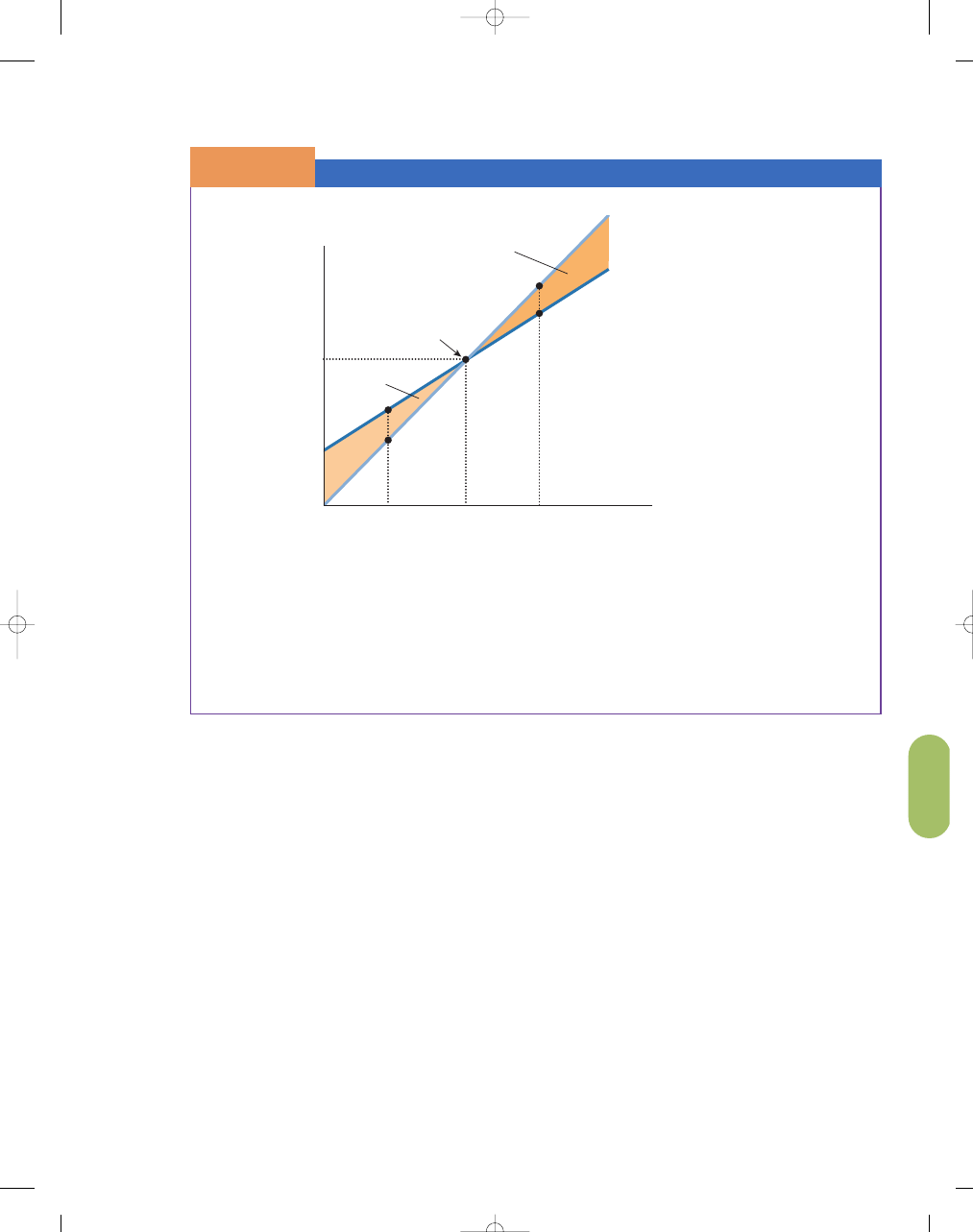
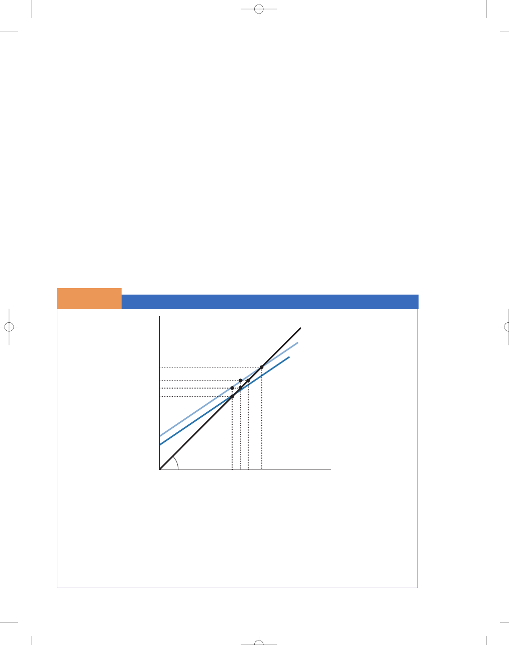
Disequilibrium and Equilibrium In the Keynesian Model

S E C T I O N

2 6 . 2

X H I B I T

When RGDP is Y

, aggregate expenditure is greater than output—distance AB on the graph. Consumers are

trying to buy more goods and services (A) than are being produced (B), which causes producers to increase the
amount of production, increasing output in the economy. This process continues until output reaches its equilib-
rium level, where the two lines intersect. If RGDP is at Y

, aggregate expenditure (D) is less than output (C).

Consumers wouldn’t want to buy all the output that is being produced, so producers would want to reduce their
production. They would keep reducing their output until the equilibrium level of output was reached. The only
point for which consumption spending equals real aggregate planned expenditure equals output is the point
where those two lines intersect. Because these points are on the 45-degree line, equilibrium output equals equi-
librium aggregate expenditure.

Real GDP, Y

Equilibrium

Spending > Output

Output > Spending

= AE

Aggregate expenditure

= Consumption

[$1 trillion

+ (0.75 × output)]

$1 trillion

$4 trillion

Real Ag

gregate Expenditure

95469_26_Ch26_p719-752.qxd 14/1/07 3:00 PM Page 725

726

M O D U L E 6

Macroeconomic Foundations

Now we can complicate our model in another impor-
tant way by adding in the other three major compo-
nents of expenditure in the economy: investment,
government purchases, and net exports. As a first
step, we’ll add these components to the model but
assume that they are autonomous, that is, they don’t

depend on the level of income or output in the econ-
omy. Later, we’ll relax that assumption.

Suppose that consumption depends on the level

of income or output in the economy, but investment,
government purchases, and net exports don’t;
instead, they depend on other things in the economy,

S E C T I O N

C H E C K

The magnitude of change in consumption spending due to a change in income is the marginal propensity to consume

(MPC); change in consumption divided by change in disposable income.

The counterpart of the marginal propensity to consume is the marginal propensity to save (MPS); the additional

savings realized as a result of a change in income. MPS equals the change in saving divided by the change in dispos-

able income.

When the Keynesian expenditure model is in equilibrium, income equals output and aggregate expenditure equals output.

Income equals output because individuals earn income through production.

Aggregate expenditure equals output because income is earned when goods and services are sold.

If consumption purchases rise with disposable income, how would an increase in taxes affect consumption purchases?

If your marginal propensity to consume was 0.75, what is your marginal propensity to save? If your marginal

propensity to consume rose to 0.80, what would happen to your marginal propensity to save?

Could a student have a positive marginal propensity to save, and yet have negative savings (increased borrowing)

at the same time?

What would happen to the slope of the consumption function if the marginal propensity to save fell?

Why would an increase in disposable income increase induced consumption but not autonomous consumption?

What tends to happen to inventories if aggregate expenditures exceed output? What tends to happen to output?

What tends to happen to inventories if output exceeds aggregate expenditures? What tends to happen to output?

What would equilibrium output be if autonomous consumption was $2 trillion and the marginal propensity to consume

was 0.75?

What would equilibrium output be if autonomous consumption was $2 trillion and the marginal propensity to consume

was 0.80?

S E C T I O N

26.3

A d d i n g I n v e s t m e n t , G o v e r n m e n t
P u r c h a s e s , a n d N e t E x p o r t s

■

What is the impact of adding investment,
government purchases, and net exports to
aggregate expenditures?

■

What is planned investment?

■

What is unplanned investment?

■

How does the Keynesian model help
explain the process of the business cycle?

= AE). The only point for which consumption

spending equals aggregate expenditure equals output
is the point where those two lines intersect, labeled

“Equilibrium.” Because these points are on the 45-
degree line, equilibrium output equals equilibrium
aggregate expenditure.

95469_26_Ch26_p719-752.qxd 14/1/07 3:00 PM Page 726

C H A P T E R 2 6

The Keynesian Expenditure Model

727

such as interest rates, political considerations, or the
condition of foreign economies (we’ll discuss these
things in more detail later). Now, aggregate expen-
diture (AE) consists of consumption (C) plus invest-
ment (I) plus government purchases (G) plus net
exports (NX):

≡ C + I + G + NX

This equation is nothing more than a definition (indi-
cated by the

≡ rather than =): Aggregate expenditure

equals the sum of its components.

When we add up all the components of aggregate

expenditure, we’ll get an upward-sloping line, as we
did in the previous section, because consumption
increases as income increases. But because we’re now
allowing for investment, government purchases, and
net exports, the autonomous portion of aggregate
expenditure is larger. Thus, the intercept of the aggre-
gate expenditure line is higher, as shown in Exhibit 1.

What is the new equilibrium? As before, the equi-

librium occurs where the two lines cross, that is, where
the aggregate expenditure line intersects the equilib-
rium line, which is the 45-degree line. We can find
the numerical value of output using some algebra as
we did before. The intersection of the two lines in the

exhibit means that aggregate expenditure, $2 trillion

(0.75

× Y), equals output, Y. So we have $2 trillion +

(0.75

× Y) = Y. Subtracting 0.75 × Y from both sides

of the equation yields $2 trillion

= 0.25Y and then

multiplying each side of the equation by 4 yields
Y

= $8 trillion.

Now that we’ve added in the other components

of spending, especially investment spending, we can
begin to discuss some of the more realistic factors
related to the business cycle. This discussion of what
happens to the economy during business cycles is a
major element of Keynesian theory, which was
designed to explain what happens in recessions.

If you look at historical economic data, you’ll

see that investment spending fluctuates much more
than overall output in the economy. In recessions,
output declines, and a major portion of the decline
occurs because investment falls sharply. In expan-
sions, investment is the major contributor to eco-
nomic growth. The two major explanations for the
volatile movement of investment over the business
cycle involve planned investment and unplanned
investment.

The first explanation for investment’s strong busi-

ness cycle movement is that planned investment
responds dramatically to perceptions of future changes
in economic activity. If business firms think that the
economy will be good in the future, they’ll build new
factories, buy more computers, and hire more workers
today, in anticipation of being able to sell more goods
in the future. On the other hand, if firms think the
economy will be weak in the future, they’ll cut back on
both investment and hiring. Economists find that
planned investment is extremely sensitive to firms’ per-
ceptions about the future. And if firms desire to invest
more today, it generates ripple effects that make the
economy grow even faster.

The second explanation for investment’s move-

ment over the business cycle is that businesses
encounter unplanned changes in investment as well.
The idea here is that recessions, to some extent, occur
as the economy is making a transition, before it reaches
equilibrium. We’ll use Exhibit 2 to illustrate this idea. In
the exhibit, equilibrium occurs at output of Y

. Now,

consider what would happen if, for some reason, firms
produced too many goods, bringing the economy to
output level Y

. At output level Y

, aggregate expendi-

ture is less than output because the aggregate expenditure
line is below the 45-degree line at that point. When
people aren’t buying all the products that firms are pro-
ducing, unsold goods begin piling up. In the national
income accounts, unsold goods in firms’ inventories
are counted in a subcategory of investment—inventory

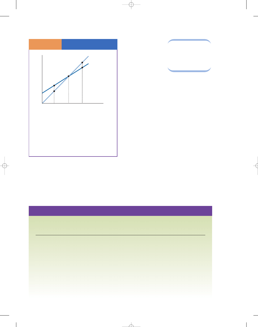
Adding Investment,
Government Purchases,
and Net Exports to
Aggregate Expenditures

S E C T I O N

2 6 . 3

X H I B I T

Adding I

+ G + NX leads to a larger intercept of the

aggregate expenditure line. Because consumption is
the only component of aggregate expenditure that
depends on income, the slope of the line is the same
as the slope of the line in Exhibit 3 of Section 26.2.
The new equilibrium occurs where the two lines cross,
where the aggregate expenditure line, which has a
slope of 0.75, intersects the equilibrium line, which is
the 45-degree line.

RGDP, Y

(trillions of dollars)

RGDP

Equilibrium

point

= C + I + G + NX

= C

= AE

Real Ag

gregate Expenditure

(trillions of dollar

95469_26_Ch26_p719-752.qxd 14/1/07 3:00 PM Page 727

728

M O D U L E 6

Macroeconomic Foundations

investment. The firms didn’t plan for this to happen,
so the piling up of inventories reflects

unplanned

inventory investment.

Of course, once firms realize

that inventories are rising because they’ve produced
too much, they cut back on production, reducing

output below Y

. This

process continues until
firms’ inventories are
restored to normal levels
and output returns to Y

Now let’s look at

what would happen if
firms produced too few
goods, as occurs when output is at Y

. At output level

, aggregate expenditure is greater than output

because the aggregate expenditure line is above the
45-degree line at that point. People want to buy more
goods than firms are producing, so firms’ inventories
begin to decline or become depleted. Again, this
change in inventories shows up in the national
income accounts, this time as a decline in firms’
inventories and thus a decline in investment. Again,
the firms didn’t plan for this situation, so once they
realize that inventories are declining because they
haven’t produced enough, they’ll increase production
beyond Y

. Equilibrium is reached when firms’ inven-

tories are restored to normal levels and output
returns to Y

So, our Keynesian expenditure model helps to

explain the process of the business cycle, working
through investment. Next, let’s see how other eco-
nomic events can act to affect the equilibrium level of
output in the economy. We’ll begin by looking at how
changes in autonomous spending (consumption,
investment, government purchases, and net exports)
can influence output.

S E C T I O N

C H E C K

Aggregate expenditure consists of consumption (C), investment (I), government expenditures (G), and net exports

(NX). Hence, in the Keynesian expenditure model, output is the result of these components.

Changes in planned or unplanned investment contribute to the fluctuations evident in the business cycle.

When all the nonconsumption components of aggregate expenditures are autonomous, why does the aggregate

expenditures line have the same slope as the consumption function?

If net exports are negative, what happens to the aggregate expenditures line, other things equal? What will happen

to equilibrium income?

If autonomous consumption is $2 trillion, investment purchases plus government purchases plus net exports is also

$2 trillion, and the marginal propensity to consume is 0.75, what is equilibrium income?

If autonomous consumption is $2 trillion, investment purchases plus government purchases plus net exports is also

$2 trillion, and the marginal propensity to consume is 0.5, what is equilibrium income?

As the economy turns toward a recession, what happens to unplanned inventory investment? Why? What happens

to planned investment? Why?

How does unplanned inventory investment signal which way real income will tend to change in the economy?

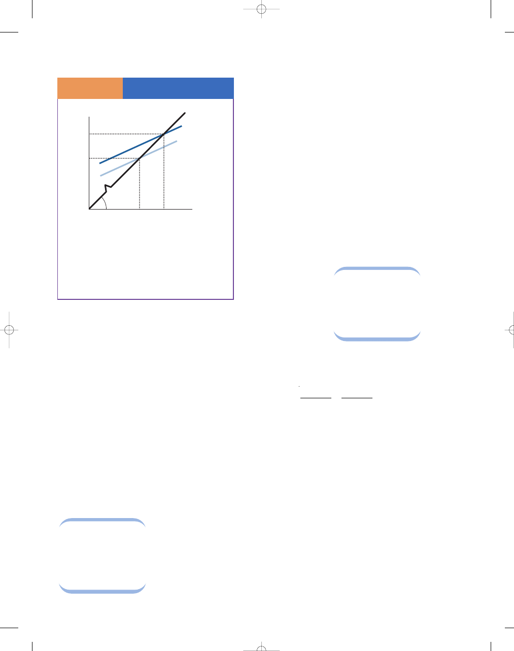
Unplanned Inventory
Investment

S E C T I O N

2 6 . 3

X H I B I T

At Y

, AE is less than output and unsold goods pile up.

As unplanned inventory investment builds up, firms cut
back on production until equilibrium output is restored
at Y

. At Y

, AE is greater than output: Consumers want

to buy more than firms are producing. Inventories
become depleted and firms increase production until
inventories are restored and output returns to equilib-
rium at Y

Real GDP, Y

(trillions of dollars)

= AE

= C + I + G + NX

Real Ag

gregate Expenditure

(trillions of dollar

)

unplanned inventory
investment

collection of inventory that results
when people do not buy the products
firms are producing

95469_26_Ch26_p719-752.qxd 14/1/07 3:00 PM Page 728

C H A P T E R 2 6

The Keynesian Expenditure Model

729

What happens if one of the components of aggregate
expenditure increases for reasons other than an increase
in income? Remember that we called these components
or parts autonomous. Households’ expectations might
become more optimistic, or households may find
credit conditions easier as interest rates decline, or
their real wealth might increase as the stock market
rises. All these factors increase autonomous consump-
tion, and thus total consumption at every level of
income increases. Firms might increase their investment
(especially if their productivity rises or the interest rate
declines), government might increase its spending, or

net exports could rise as foreign economies improve their
economic health. Any of these things would increase
aggregate expenditure for any given level of income,
shifting the aggregate expenditure curve up, as shown in
Exhibit 1.

Let’s continue with our earlier numerical example

and suppose that government purchases increased by
$500 billion because the government undertook a
large spending project, such as deciding to rebuild a
major portion of the interstate highway system. The
increase in government purchases of $500 billion
increases the autonomous portion of aggregate expen-
diture from $2 trillion to $2.5 trillion. As the exhibit
shows, the upward shift in the aggregate expenditure
curve (from AE

to AE

) leads to an equilibrium with

a higher level of output. Again, using algebra, we can
find out exactly how much the new equilibrium output
will be.

Setting aggregate

expenditure [$2.5 tril-
lion

+ (0.75 × Output)]

equal to output, we
find that output is
$10 trillion. So output
rose from $8 trillion to
$10 trillion. This result
might seem amazing—
that an increase in government spending of $500 bil-
lion can lead to a $2 trillion increase in output—but
it merely reflects a well-understood process, known as
the

expenditure multiplier.

A caution here: Do not assume that the multiplier

applies only to changes in government spending.
Multipliers apply to any increase in autonomous expen-
diture. As an example, if the stock market went up to
increase the amount of autonomous household spend-
ing by $500 billion, the level of output would go up the
same $2 trillion as found in the preceding example.

The idea of the multiplier is that permanent

increases in spending in one part of the economy lead
to increased spending by others in the economy as well.
When the government (or other autonomous compo-
nents of aggregate expenditures) spends more, private

S E C T I O N

26.4

S h i f t s i n A g g r e g a t e E x p e n d i t u r e
a n d t h e M u l t i p l i e r

■

How do changes in the components of
aggregate expenditure affect the aggregate
expenditure curve?

■

How does the multiplier affect aggregate
expenditures?

expenditure
multiplier

the multiplier that only considers
the impact of consumption changes
on aggregate expenditures

Increases in the Autonomous
Components of Aggregate
Expenditure

S E C T I O N

2 6 . 4

X H I B I T

If one of the “autonomous” components of aggre-
gate expenditure increases for reasons other than
an increase in income like: optimistic consumer
or business expectations, a decrease in the interest
rate, real wealth increases, government might
increase its spending, or net exports could rise as
foreign economies improve their economic health.
Any of these things would increase aggregate
expenditure for any given level of income, shifting
the aggregate expenditure curve up, as shown in
Exhibit 1.

Real GDP, Y

(trillions of dollars)

= $2.5 trillion +

(0.75

× Output)

= $2 trillion +

(0.75

× Output)

Y = AE

2.5

Real Ag

gregate Expenditure

(trillions of dollar

95469_26_Ch26_p719-752.qxd 14/1/07 3:00 PM Page 729

730

M O D U L E 6

Macroeconomic Foundations

citizens earn more wages, interest, rents, and profits,
so they spend more. The higher level of economic
activity encourages even more spending, until a new
equilibrium with higher output is reached. In this
example, the increase in output is four times as big as
the initial increase in government spending that
started the cycle. Let’s see how this process works in
more detail.

Suppose, as in Exhibit 1, that we are initially in

equilibrium at point A, with output of $8 trillion. Just
as in the example, let’s suppose that the government
increases spending by $500 billion, so we know that
we’ll eventually get to a new equilibrium at point Z in
the exhibit, with output of $10 trillion. Now let’s see
how we get from point A to point Z, with just induced
consumer spending propelling the economy along.

Exhibit 2 shows what happens along the way. We

begin at point A, with output of $8 trillion. The
increase in government purchases of $500 billion

directly increases aggregate expenditure by that
amount, represented by point B. Firms observe the
increase in aggregate expenditure (perhaps because
they see their inventories declining), so over the next
few months they produce more output, moving the
economy to point C, with output of $8.5 trillion. But
now consumers have an extra $500 billion in income
and they wish to spend three-fourths of it (because the
marginal propensity to consume is 0.75). Three-fourths
of $500 billion is $375 billion, so consumers now
spend an additional $375 billion, increasing aggregate
expenditure to $8.875 trillion at point D. Again,
firms observe the increase in expenditure, so over
the next few months they increase output, bringing
the economy to point E. This process continues
until the economy eventually reaches point Z, at which
output is $10 trillion. Notice that the process is not
accomplished immediately, but over several quarters
of time.

Aggregate Expenditures and the Multiplier Process

S E C T I O N

2 6 . 4

X H I B I T

At point A, output is $8 trillion and the increase in government purchases of $500 billion directly increases aggregate
expenditure by that amount, represented by point B. Firms observe the increase in aggregate expenditure and pro-
duce more output, moving the economy to point C, with output of $8.5 trillion. But now consumers have an extra
$500 billion in income and they wish to spend three-fourths of it (the MPC is 0.75). Three-fourths of $500 billion is
$375 billion, so consumers now spend an additional $375 billion, increasing aggregate expenditure to $8.875 trillion
at point D. Again, firms observe the increase in expenditure and increase output bringing the economy to point E.
This process continues until the economy eventually reaches point Z, at which output is $10 trillion. The process is not
accomplished immediately, but over several quarters of time.

RGDP, Y

(trillions of dollars)

= $2.5 trillion +

(0.75

× Output)

= $2 trillion +

(0.75

× Output)

Y = AE

8.5

8.875

2.5

8.5

8.875

Real Ag

gregate Expenditure

(trillions of dollar

95469_26_Ch26_p719-752.qxd 14/1/07 3:00 PM Page 730

C H A P T E R 2 6

The Keynesian Expenditure Model

731

You can see on the graph how the economy

reaches its new equilibrium at point Z. We can also
calculate it numerically by adding up an infinite series
of numbers in the following way. The first increase in
output was $500 billion, which comes directly from
the increase in government purchases. Then con-
sumers, with higher incomes of $500 billion, want to
spend three-fourths of it, so they increase spending:
$500 billion

× 3/4 = $375 billion. Now, with incomes

higher by $375 billion, consumers want to spend an
additional three-fourths of it: $375 billion

× 3/4 =

$281.25 billion. Again, incomes are higher, so con-
sumers will spend more, this time in the amount
$281.25

× 3/4 = $210.94 billion. The process contin-

ues indefinitely. To find the total increase in output
(or income), we simply need to add up all these
amounts. They total $500 billion

+ $375 billion +

$281.25 billion

+ $210.94 billion + . . . . The process

goes on infinitely, but fortunately, the sum of the num-
bers is finite, as we can see using algebra. Notice that
to get these numbers, we started with $500 billion,
then took 3/4

× $500 billion (to get $375 billion), then

multiplied that amount by 3/4 (to get $281.25 billion),
and so on. So the increase in output

= $500 billion +

(3/4

× $500 billion) + (3/4 × 3/4 × $500 billion) + (3/4 ×

3/4

× 3/4 × $500 billion) + . . . . It turns out that an

infinite sum with this pattern is exactly $500 billion/
(1

− 3/4) = $2 trillion. So output increases by $2 trillion,

from $8 trillion to $10 trillion.

This calculation of the sum of all the increases to

output can be written in a more convenient way.
Following the same process we just used, whenever an
autonomous element of spending increases by some
amount, output in the economy rises by that amount
times the multiplier. As you saw in this example, the
multiplier depends on how much consumers spend
out of any additions to their income. So in this model
in which consumption spending is the only compo-
nent of aggregate expenditure that depends on
income, the multiplier is equal to 1/(1

− MPC), where

MPC is the marginal propensity to consume. In the
previous example, MPC

= 3/4, so the multiplier is

1/(1

− 3/4) = 4. The same multiplier holds whether the

increase in aggregate expenditures arises from an
increase in government purchases, as in the example,
or from an increase in other autonomous elements
of spending, such as investment, net exports, or the
autonomous portion of consumption spending. The mul-
tiplier just developed was designed to provide insights
into the process of how it works. The actual multi-
plier for the U.S. economy is thought to be about half
this size, about 2.

S E C T I O N

C H E C K

Autonomous changes in the components of aggregate expenditure change the total level of aggregate expenditure,

and thus output.

The effect of spending in one part of the economy is magnified by the multiplier and can affect the other compo-

nents; the change in output may be greater than the change in spending.

Where consumption spending is the only variable of aggregate expenditure dependent on income, the multiplier

is 1

/(1 − MPC).

If autonomous expenditure rises and the marginal propensity to consume rises, what would happen to equilibrium

income?

If autonomous expenditure rises and the marginal propensity to consume falls, what would happen to equilibrium

income?

If the marginal propensity to consume was 0.75, what would happen to equilibrium income if government purchases

increased by $500 billion and investment fell by $500 billion at the same time? What if government purchases increased

by $500 billion and investment fell by $400 billion at the same time?

Why does a larger marginal propensity to consume lead to a larger multiplier?

If autonomous consumption was $300 billion, investment was $200 billion, government purchases were $400 billion,

and net exports were a negative $100 billion, what would autonomous consumption be? What would equilibrium

income be?

What would happen to equilibrium income if, other things equal, imports increased by $100 billion and the marginal

propensity to consume was 0.9?

95469_26_Ch26_p719-752.qxd 14/1/07 3:00 PM Page 731

732

M O D U L E 6

Macroeconomic Foundations

In developing the Keynesian expenditure model, we
simplified many elements of the economy. We assumed
that the only element of aggregate expenditure that
depended on income was consumption, and that all
the other components were autonomous. Now that
this simpler model has been presented, we can compli-
cate the model in many ways, but the intuition under-
lying equilibrium and the calculation of the multiplier
remain the same.

First, consider investment spending. Economists

studying investment spending have found that it
depends on people’s expectations of future economic
conditions, taxes, interest rates, and the size of the
current capital stock compared to the desired capital
stock. Could investment spending also depend on cur-
rent income? It might, especially if firms view the
change in current income as an indicator of future
changes in income. Furthermore, given a firm’s cost
structure, an increase in current income may generate
profits or cash flows that can be used for financing
investment expenditures. In this case, an increase in
income would increase their ability to invest, so
investment would rise.

Government purchases also might be directly

affected by current income in the economy. Although
the process for determining the federal government
budget is slow and deliberate and constitutes what is
known as fiscal policy, state and local governments
often have balanced-budget requirements. To balance
their budgets, state and local governments often
reduce their spending in recessions as tax revenues
fall, and can afford to increase their spending in
expansions as tax revenue rises. So to some extent,
part of government purchases may be affected by cur-
rent income.

Finally, net exports are strongly dependent on a

country’s income, as well as other factors, such as
exchange rates between the currencies and price levels
in different countries. Holding the rest of the world
constant, when an economy is growing strongly, with
rising income, it imports more goods from other coun-
tries. When an economy is in recession, with falling
income, it imports less. As a result, an economy with

high income has lower net exports, while an economy
with low income has higher net exports. So net exports
are also influenced by the economy’s current income.
But notice that the direction is the opposite of the rela-
tionship between the other components of aggregate
expenditure and income. Consumption, investment,
and government purchases are all positively related
with income (when income rises, they rise) but net
exports are negatively related to income.

Why is the relationship of all these elements of

aggregate expenditure with income so important? The
relationship affects the multiplier. Remember that the
multiplier in the earlier example (in which consump-
tion was the only component that depended on
income) was equal to 1/(1

− MPC), where MPC is the

marginal propensity to consume. When we allow the
other components of aggregate expenditure to depend
on income, as described here, the same logic behind
the multiplier holds, but the formula changes slightly.
The multiplier is now 1/(1

− MPAE), where MPAE is

the marginal propensity of aggregate expenditure,
which in turn is equal to the marginal propensity to
consume out of disposable income (the change in dis-
posable income as total income changes) plus the
marginal propensity to invest (which is the amount
that investment increases when income rises) plus the
marginal propensity of government purchases (the
amount that government purchases increase when
income rises) minus the marginal propensity to
import (the amount that imports increase when
income rises). Notice that the marginal propensity
to import enters with a minus sign because imports
are goods that aren’t produced within the country.
The final result of this modification is to make the
MPAE approximately equal to 0.5. Placing this
value in our multiplier formula results in a multi-
plier no larger than 2.

Now we have a more complicated model, but we

don’t always need to use the more complicated
approach. Economists have found that it’s often best
to use the simplest model possible, the one that gets at
the essentials and ignores the less-important elements,
when solving an economic problem.

S E C T I O N

26.5

A C o m p l e t e M o d e l

■

Does investment spending depend on
current income?

■

How do government purchases affect
current income?

■

How does income impact net exports?

■

What is the marginal propensity of aggregate
expenditures?

95469_26_Ch26_p719-752.qxd 14/1/07 3:00 PM Page 732

C H A P T E R 2 6

The Keynesian Expenditure Model

733

The Keynesian expenditure model is often used to pro-
vide insight into changes in fiscal policy, the counter-
cyclical expenditure and tax policy of the federal
government. We will study the role of fiscal policy as
a countercyclical tool in the next chapter.

Earlier, we developed the multiplier based on a

change in autonomous government purchases. Now,
we want to see what happens when taxes change.
Finally, we want to examine balanced-budget changes
that occur when the government changes both spend-
ing and taxes by the same amount. (Since the possi-
bility that government purchases might depend on
income doesn’t matter for what we’re going to do,
we’ll return to the simple model in which only con-
sumption depends on income.)

First, let’s see what happens if the government

increases taxes by some amount, say $100 billion. We
are thinking of taxes, an amount of dollars paid that
is often called lump-sum taxes or fixed taxes, that is,

taxes that do not depend on the level of income. We’ll
assume that consumers pay the taxes, so the effect of
the tax increase is just like a reduction in consumers’
incomes. How much will consumers reduce their
spending? Because the tax increase is like a reduction
in income, consumers will reduce their spending by
the amount of the tax increase times the marginal
propensity to consume. If the marginal propensity to
consume is three-fourths, as in the example we dis-
cussed earlier, then consumers will reduce their spend-
ing by $75 billion. Thus, aggregate expenditure will
decline by $75 billion because of the direct impact of
the higher taxes. And what will happen in equilib-
rium? As Exhibit 1 shows, with aggregate expenditure
of $75 billion less, the new equilibrium level of output
is lower by the multiplier (4) times the change in aggre-
gate expenditure ($75 billion), which equals $300 bil-
lion. So output in the economy declines from $8 trillion
to $7.7 trillion.

S E C T I O N

C H E C K

In a more complex model, the components of aggregate expenditure in addition to consumption (investment,

government expenditure, and net exports) are influenced by current income.

Consumption, investment, and government expenditures are related positively to income; net exports are nega-

tively related.

When all the factors of aggregate expenditure are influenced by income, the multiplier becomes a function of the mar-

ginal propensity of aggregate expenditure (MPAE) rather than MPC. In this case, the multiplier equals 1

/(1 − MPAE).

If investment as well as consumption increased with income, for a given level of autonomous expenditures, what

will happen to equilibrium income?

If consumption fell, beginning a recession, but local government purchases also fell as a result, how would that

affect the resulting change in equilibrium income?

What will growth in U.S. income do to net exports?

What is MPAE if the marginal propensity to consume was 0.5, the marginal propensity to invest was 0.1, the marginal

propensity of government purchases was 0.2, and the marginal propensity to import was 0.05?

What would happen to the multiplier if the marginal propensity to consume went up and the marginal propensity

to invest went down at the same time?

S E C T I O N

26.6

G o v e r n m e n t P u r c h a s e s , Ta x e s ,
a n d t h e B a l a n c e d - B u d g e t M u l t i p l i e r

■

What happens if the government increases
taxes?

■

What is the difference between the multi-
plier on taxes and government purchases?

■

What is the balanced-budget multiplier?

95469_26_Ch26_p719-752.qxd 14/1/07 3:00 PM Page 733

734

M O D U L E 6

Macroeconomic Foundations

So, just as a multiplier effect influences govern-

ment purchases, the same thing happens with taxes.
But the two cases are different in an important way.
When we looked at an increase in government pur-
chases, we found that output changed in the same
direction by the multiplier times the change in gov-
ernment purchases. But in the case of an increase in
taxes, output changes in the opposite direction by the
multiplier times an amount equal to the marginal
propensity to consume times the change in taxes. In
the example, the tax increase of $100 billion caused
aggregate expenditure to decline by 3/4

× $100 billion,

which equals $75 billion. So a change in taxes of a
given amount affects aggregate expenditure by less
than that amount, because the marginal propensity to
consume is less than 1.

This fact means that when the government

changes both government purchases and taxes by
the same amount, an event that some economists

call a

balanced-budget

change in fiscal policy,

output is still affected.
We use the term, bal-
anced budget, to call
attention to the fact
that both taxes and
government expendi-
tures change by the same
amount. For example, if

the government increases its purchases by $100 billion
and pays for the increased purchases by raising
$100 billion of additional taxes, the increase in gov-
ernment purchases increases aggregate expenditure
by $100 billion, but the increase in taxes reduces
aggregate expenditure by only 3/4

× $100 billion =

$75 billion. So the net effect is an increase in aggre-
gate expenditure of $25 billion. With a marginal
propensity to consume of three-fourths, the mul-
tiplier is 4, so the total impact on output is 4

$25 billion

= $100 billion. Similarly, a balanced-

budget decrease in government purchases and an
equivalent decrease in taxes of $100 billion would
lead to a reduction in aggregate expenditure of
$25 billion, which would lead to a decline in output
of $100 billion.

Because the change in government purchases

increases output by the multiplier times the change
in purchases, while a change in taxes decreases
output by the multiplier
times the change in
taxes times the marginal
propensity to consume,
the

balanced-budget

multiplier

is less than

the multiplier we used
before (which we’ll call
the basic expenditure
multiplier from now on).
In fact, if the basic expenditure multiplier is equal to
1/(1

− MPC), the balanced-budget multiplier is

1/(1

− MPC) reflects the effect of government pur-

chases on aggregate expenditure, and MPC/(1

− MPC)

reflects the effect of taxes on aggregate expenditure.
The result of the equation equals exactly 1. So the
balanced-budget multiplier is equal to 1, no matter
what the marginal propensity to consume. Thus, as we
saw in our example, a balanced-budget increase in
government purchases (and taxes) of $100 billion
increases output by $100 billion, while a balanced-
budget decrease in government purchases (and taxes)
of $100 billion decreases output by $100 billion.

We’ve now developed the Keynesian expenditure

model in complete detail. It’s a useful model for exam-
ining what happens to output in the economy when
changes occur in the autonomous components of
aggregate expenditure. But the Keynesian expenditure
model is not a complete macroeconomic model, as
we’ll now see.

(

−

MPC)

MPC

MPC)

Aggregate Expenditures
and a Tax Cut

S E C T I O N

2 6 . 6

X H I B I T

Aggregate expenditure declines by $75 billion as a
result of higher taxes. The new equilibrium level of
output is lower by the multiplier (4) times the change
in aggregate expenditure ($75 billion), which equals
$300 billion. So output in the economy declines from
$8 trillion to $7.7 trillion.

balanced-budget
change in fiscal
policy

policy in which the government
changes both government expendi-
tures and taxes by an equal amount

balanced-budget
multiplier

a multiplier that reflects the effect
of government purchases and tax
changes on aggregate expenditures,
and is thus equal to 1

Y = AE

= $2,000 billion

+ (0.75

× Output)

= $1,925 billion

+ (0.75

× Output)

gregate Expenditure

(trillions of dollar

Real GDP, Y

(trillions of dollars)

7.7

95469_26_Ch26_p719-752.qxd 14/1/07 3:00 PM Page 734

C H A P T E R 2 6

The Keynesian Expenditure Model

735

Suppose all households in aggregate decide to save an
extra $5 billion this year, instead of spending it. This
kind of change would be an autonomous change in
tastes or it could be triggered by a change in auto-
nomous expectations as discussed earlier. Returning
to our previous numerical example, we assume the
marginal propensity to consume is 3/4 and the multi-
plier is 4. Under these assumptions, the increased
saving of $5 billion leads to a decrease in consump-
tion spending of $5 billion, which in turn leads to a
decrease of $5 billion

× 4 = $20 billion in the nation’s

output. This result seems strange, doesn’t it? People
often believe that saving is a virtue, yet in this model,
saving reduces the economy’s output. The paradox is
that thrift is desirable for any individual or family, but
it might cause problems for the economy as a whole.

WHAT THE KEYNESIAN EXPENDITURE
MODEL IS MISSING

The paradox of thrift helps point out a key, missing
ingredient of the Keynesian expenditure model. When
saving rises, the economy should experience some ben-
efit, yet the model suggests that the only result is a

decline in output. The Keynesian expenditure model
clearly shows that when people make decisions about
spending, they influence the amount of demand in the
economy, but what’s missing is the notion of supply.

To see the importance of adding the idea of supply

to the model, again suppose the multiplier is 4. Then if
the government (or households or business firms)
increased its spending by $1 trillion, the economy’s
output would rise by $4 trillion. But why doesn’t the
government increase spending by $2 trillion so the econ-
omy’s output would rise by $8 trillion? Why doesn’t the
government simply raise output infinitely? Government
revenue (or the size of the deficit) faces some con-
straints, where eventually all taxes or deficits have to be
approved by Congress and ultimately the citizens of the
country. But the essential reason the government (or any
other sector, households or firms) can’t do this in reality
is that output is limited by scarce resources. The gov-
ernment can raise aggregate expenditure by increasing
its spending, but for output to go up, something must
cause an increase in aggregate supply. For this reason,
the Keynesian expenditure model is best seen as a model
of aggregate demand and not a complete model of the
economy.

S E C T I O N

26.7

T h e P a r a d o x o f T h r i f t

■

What is the paradox of thrift?

■

What are the implications for not including
the notion of supply?

S E C T I O N

C H E C K

Tax increases are similar to a reduction in income, decreasing aggregate expenditure and output.

Because of the marginal propensity to consume, changes in taxes of a given amount affect aggregate expenditure

by less than the change in taxes, which explains why output changes when the government alters its expenditures

and taxes by equal amounts.

The balanced-budget multiplier reflects the effect of government purchases and tax changes on aggregate expenditures,

and is thus equal to 1.

If government purchases rise by $10 million and the marginal propensity to consume is 0.75, what happens to equilibrium

income? If taxes fall by $10 million, what happens to equilibrium income?

Why will the effect on autonomous consumption of a given change in taxes equal minus the marginal propensity to

consume times the effect of an equal change in government purchases?

If a change in equilibrium income was equal to the change in government purchases that caused it, why do we

know that the government funded the increase in purchases with an equal increase in taxes?

95469_26_Ch26_p719-752.qxd 14/1/07 3:00 PM Page 735

736

M O D U L E 6

Macroeconomic Foundations

i n t h e n e w s

Japan’s Paradox of Thrift

A decade ago, when Japan was considered economically mighty and the
United States was struggling, many economists agreed that a big reason for
the disparity was savings: The thrifty Japanese had plenty to invest in their
future, the wanton Americans too little.

Today, the average Japanese family puts away more than 13% of its income,

the average American family 4%. Yet Japan is in the tank while the U.S. prospers.

Is saving no longer an economic virtue and profligacy no longer a vice?

Did Benjamin Franklin get it all wrong? Maybe not—but it isn’t as simple as
Franklin’s Poor Richard’s Almanac made it seem:

■

An economy can save too much.

Japan is the first major developed country since World War II to confront the
“paradox of thrift,” the condition John Maynard Keynes worried about, where
bad times lead individuals to save more, suppressing overall demand and
making a country even worse off.

■

As important as how much a country saves is how well those savings
are invested.

Japan today is a showcase of squandered savings, from lightly traveled
bridges to empty office towers. The U.S. is a display of scarce savings
leveraged skillfully that have transformed entire industries, such as high-
tech start-ups.

■

In an era of global financial markets, a country that doesn’t save enough
on its own can live off other countries’ savings for a long time.

“People who just focused on savings rates missed two things,” says Stanford
University economist Michael Boskin. “They assumed all savings was produc-
tively invested, and they viewed foreign investment as necessarily evil.” But,
he adds, “focusing just on savings is like saying you have to have good tires to
go fast. You also need a good engine.”

Most economists say that national savings—the combined savings of

households, businesses, and governments—does matter. If two economies are
similar in other respects, the one with higher savings will almost always be
better off, they say. In the long run, they warn, America’s savings dearth
threatens the living standards of future generations.

But these days, the pressing savings crisis is in Tokyo. Interest rates on

bank deposits run below 1%, and still “households are saving too much,”
says Kengo Inoue, a Bank of Japan economist. “That’s depressing demand
and, over time, corporate investment.” That, in turn, has become a drag on
all of Asia.

So the Japanese government nudges its citizens to live it up. The

Finance Ministry, concerned that families would simply tuck away a recent

$500-a-household income-tax cut, launched a media blitz to advise people on
how to spend the money.

A cartoon in a magazine ad shows a father excitedly reading about the

cuts in the newspaper, inspiring his two young kids to dream of cake and
candy and his blushing wife to ask for a blouse. A poster plastered in subway
stations pictures an aerial shot of a crammed neighborhood with words
emanating from the homes. “I’ll drink a toast with fine wine,” says one. “I’ll
finally buy those golf clubs,” says another. One implores: “Let’s spend it all
at once!”

Such an emphasis on savings “is a social, moral policy, as well as an eco-

nomic policy,” says Sheldon Garon, a Princeton University professor and
expert on Japanese history. “When Japanese talk about themselves, they say
they’re more thrifty than others, than Americans.”

Muses Hideaki Kase, an influential conservative writer: “Now we are being

told that you have to spend to maintain the vitality of society. But frugality has
been a major strength of the nation. Why are we great savers? That’s like
asking Japanese, ‘Why do you breathe?’”

Government policies play a huge role. U.S. tax law encourages consumer

borrowing. Japanese law and custom, while encouraging massive corporate
borrowing, discourages household debt. U.S. homebuyers can deduct interest
payments on mortgages; Japanese get a much smaller break—as a tax credit—
for the first six years of a housing loan. And Japanese consumers are more
debt averse. MasterCard International estimates that consumers in the U.S.
pay for 30% of their total purchases via credit cards. Only 15% of Japanese con-
sumers’ expenditures go through plastic.

SOURCE: Jacob M. Schlesinger and David P. Hamilton, “Japan’s Paradox of Thrift,”

Photodisc Green/Getty Images

95469_26_Ch26_p719-752.qxd 14/1/07 3:01 PM Page 736

C H A P T E R 2 6

The Keynesian Expenditure Model

737

To go from the Keynesian-cross to aggregate demand, all
we need to add is how the price level affects the compo-
nents of aggregate demand. In everything we’ve done so
far, we implicitly assumed that the price level remained
constant, along with other financial variables (such as
the money supply) that we didn’t discuss. But now we
need to complicate the model in yet another dimension,
allowing the components of aggregate expenditure to
depend on the price level. The textbook provides three
main reasons for this dependence on price level:
(1) Consumption rises when the price level falls, because
people’s real wealth rises (the real wealth effect). Return
and reread the section on autonomous consumption.
(2) Investment rises when the price level falls because
interest rates decline (the interest rate effect). (3) Net
exports rise when the price level falls because now
domestic goods are cheaper than foreign goods, and
interest rates and the exchange rate decline (the open
economy effect).

The effect of different price levels can be seen in

Exhibit 1. Let’s consider three different price levels,
P

= 90, P = 100, and P = 110, where P is a price index

like the GDP deflator. Suppose the price level is 100,
and suppose at that level of prices, the aggregate expen-
diture curve is given as the curve labeled AE(P

= 100),

shown in the top diagram. The equilibrium in the
Keynesian expenditure model occurs at point A. Now

we plot point A in the bottom diagram, corresponding
to a price level of 100 and output of $8 trillion.

What happens if the price level falls from 100 to

90? The lower price level means higher aggregate
expenditure, so the aggregate expenditure curve shifts
up to AE(P

= 90), and the equilibrium in the Keynesian-

cross diagram is at point B. So we plot point B in the
bottom diagram, corresponding to price level 90 and
output $9 trillion.

Finally, what happens if the price level rises to 110?

The higher price level means lower aggregate expendi-
ture, so the aggregate expenditure curve shifts down to
AE(P

= 110), and the equilibrium in the Keynesian-

cross diagram is at point C. We plot point C in the
bottom diagram, corresponding to a price level of 110
and output of $7 trillion.

Notice that the higher the price level, the lower is

aggregate demand. Imagine carrying out this same
experiment for every possible price level. Then the points
like A, B, and C in the lower diagram would trace out
the entire aggregate demand curve, as shown.

SHIFTS IN AGGREGATE DEMAND

In the previous section, we used the relationship
between aggregate expenditure and the price level to
derive the aggregate demand curve. Now we’ll show

S E C T I O N

26.8

K e y n e s i a n - C r o s s t o A g g r e g a t e D e m a n d

■

Why do aggregate expenditures depend on
the price level?

■

How do we move from the Keynesian-cross
to aggregate demand?

S E C T I O N

C H E C K

Although saving is presumed to be good for individuals, the Keynesian expenditure model suggests that increased

saving reduces the economy’s output: the paradox of thrift.

The notion of aggregate supply is missing from the Keynesian expenditure model. Aggregate supply explains why

output growth through expenditure is eventually limited.

Why does an increase in autonomous saving decrease equilibrium income?

If autonomous saving and investment increased by the same amount, what would be the effect on equilibrium income?

If autonomous expenditures were $1 trillion and the marginal propensity to save increased from 0.20 to 0.25, what

would happen to equilibrium income?

Why is the Keynesian expenditure model’s assumption of a fixed price level misleading once the productive capac-

ity of the economy is reached?

95469_26_Ch26_p719-752.qxd 14/1/07 3:01 PM Page 737

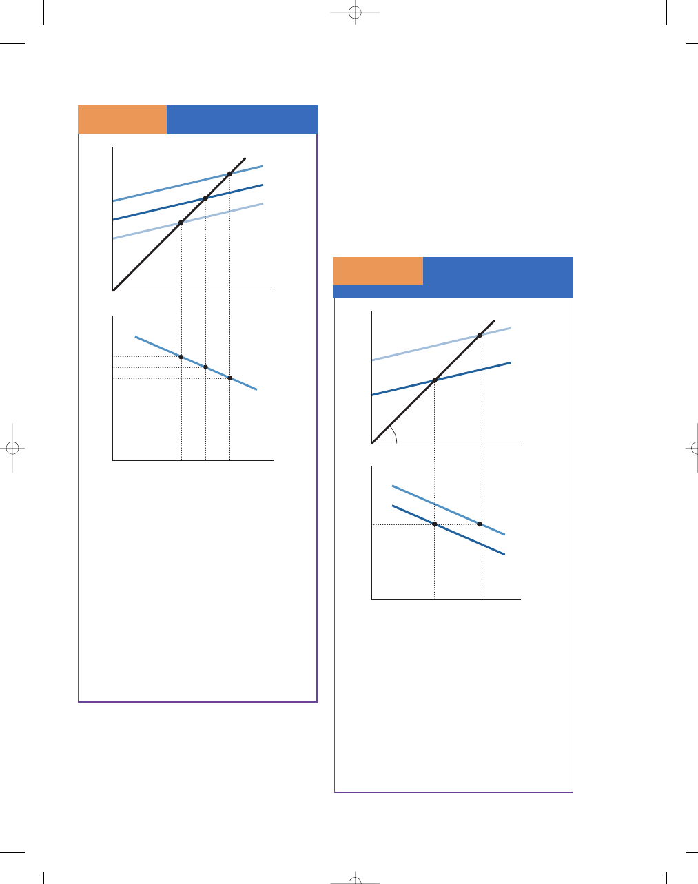
738

M O D U L E 6

Macroeconomic Foundations

that changes in any of the components of aggregate
expenditure that occur for any reason other than a
change in the price level or output lead to a shift of
the aggregate demand curve. We’ll start with Exhibit 1
(but to keep things readable we’ll only draw in one of

the aggregate expenditure lines in the top half of the
exhibit), then consider what happens when the auto-
nomous parts of consumption, investment, govern-
ment purchases, or net exports change, as we did in
Exhibit 1 from Section 26.4. Such a change would
shift the aggregate expenditure curve upwards, as
shown in Exhibit 2, where we denote the original
aggregate expenditure curve AE

and the new

aggregate expenditure curve AE

. (You can visualize a

similar shift in the other aggregate expenditure

From Aggregate Expenditure
to Aggregate Demand

S E C T I O N

2 6 . 8

X H I B I T

Suppose the price level is 100, and suppose at that
level of prices, the aggregate expenditure curve is
given as the curve labeled AE(P

= 100), shown in the

top diagram. The equilibrium in the Keynesian expen-
diture model occurs at point A. Now we plot point A
in the bottom diagram, corresponding to a price
level of 100 and output of $8 trillion. If the price
level falls from 100 to 90, the aggregate expenditure
curve shifts up to AE(P

= 90), and the equilibrium in

the Keynesian-cross diagram is at point B. So we plot
point B in the bottom diagram, corresponding to
price level 90 and output $9 trillion. If the price level
rises to 110 the aggregate expenditure curve shifts
down to AE(P

= 110), and the equilibrium is at point C.

We plot point C in the bottom diagram, correspon-
ding to a price level of 110 and output of $7 trillion.

Shifting the Aggregate
Expenditure and the
Aggregate Demand Curve

S E C T I O N

2 6 . 8

X H I B I T

If the autonomous parts of consumption, investment,
government purchases, or net exports change, it shifts
the aggregate expenditure curve upwards from AE

to AE

. Originally, we had equilibrium at point A with

output of $8 trillion when the price level was 100.
Now suppose the government increased spending,
the aggregate expenditure curve shifts up, and we
get equilibrium at point D with output of $8.5 trillion
when the price level is 100. Similarly, for any other
given price level, equilibrium output would be higher.
So, the new aggregate demand curve on the lower
diagram has shifted to the right.

Real GDP, Y

(trillions of dollars)

Y = AE

AE(P = 90)

AE (P = 100)

AE (P = 110)

Real Ag

gregate Expenditure

(trillions of dollar

Price Le

vel

Real GDP, Y

(trillions of dollars)

110
100

Aggregate

Demand

Real GDP, Y

(trillions of dollars)

Y = AE

(P = 100)

Real Ag

gregate Expenditure

(trillions of dollar

)

Price Le

vel

Real GDP, Y

(trillions of dollars)

100

8.5

95469_26_Ch26_p719-752.qxd 14/1/07 3:01 PM Page 738

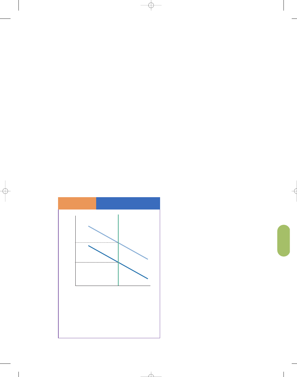
C H A P T E R 2 6

The Keynesian Expenditure Model

739

curves, corresponding to P

= 90 and P = 110, drawn

in Exhibit 1.)

Originally, we had equilibrium at point A with

output of $8 trillion when the price level was 100.
After the increase in government spending, the
aggregate expenditure curve shifts up, and we get
equilibrium at point D with output of $8.5 trillion
when the price level is 100. Similarly, for any other
given price level, equilibrium output would be higher.
So, the new aggregate demand curve on the lower dia-
gram has shifted to the right.

The aggregate demand curve can now be combined

with a model of aggregate supply in the economy, as dis-
cussed in greater detail in Chapter 25. As an example,
suppose the aggregate supply curve is vertical, as it must
be in the long run, because the price level has no long-
lasting effect on output. Now, consider our example of
an increase in government purchases (or any other
autonomous change). As shown in Exhibit 3, the origi-
nal aggregate demand curve is AD

and the increase in

government purchases shifts the aggregate demand
curve to AD

. What happens to output? It is unchanged

from its original level. A rise in the price level from
100 to 105 is the only effect of the higher level of gov-
ernment expenditures. In this case, the expenditure

multiplier effect on real output (RGDP) is zero. Changes
in aggregate expenditure lead to no increase in output.
Try this exercise with a different autonomous change
such as wealth or expectations.

As the textbook explains in more detail, in the

short run the aggregate supply curve slopes upward, so
an increase in aggregate expenditure will lead to some
increase in output in the short run. In that case, the
effect on real output in the short run will be greater
than zero, but not as large as the basic expenditure
multiplier, 1/(1

− MPC), which we derived without con-

sidering the effects of aggregate supply.

So the important point is that supply considera-

tions are important in constraining the impact of a
change in aggregate expenditure on output.

THE KEYNESIAN SHORT-RUN AGGREGATE SUPPLY
CURVE—STICKY PRICES AND WAGES

Keynes and his followers argued that wages and price
are inflexible downward. As we discussed in Chapter 25,
wage stickiness can arise as a result of long-term labor
and raw material contracts, unions, and minimum wage
laws. If wages and prices are sticky and the economy has
sufficient excess capacity, then the short-run aggregate
supply curve is flat, because full employment of all
resources is not reached until RGDP

. That is, with so

many resources idle, producers will not have to compete
with each other for machinery or labor and input prices
will tend to stay flat.

In Exhibit 4, we see that in the flat portion of the

SRAS curve an increase in AD from AD

to AD

has

little impact on the price level but considerable impact
on real GDP and employment. When AD

increases

to AD

, we see an increase in real gross domestic

product from RGDP

to RGDP

—a new equilibrium

where resources are more fully utilized. Similarly, a
reduction in AD in this region will also leave the price
level unchanged. Specifically, it means that the price
level does not rise or fall much in this situation, but
RGDP does. This price and wage inflexibility when
AD is falling played a significant part in the
Keynesian theory. With stickiness of wages and other
input costs, a reduction in aggregate demand will not
lead to a lower price level if the economy has suffi-
cient excess capacity—say at RGDP

rather than

RGDP

. Historically, the mid to late 1930s seems to

fit the Keynesian model quite well—increases in
RGDP without simultaneous increases in the price
level. It was a period of high unemployment of
resources and double-digit unemployment—that is,
sufficient level of excess capacity and little competi-
tion to bid up input prices.

Aggregate Demand
and Aggregate Supply

S E C T I O N

2 6 . 8

X H I B I T

An increase in government purchases shifts the aggre-
gate demand curve from AD

to AD

. Output is

unchanged, and the price level rises from 100 to 105.
In this case, the expenditure multiplier effect on real
output (RGDP) is zero because the changes in aggre-
gate expenditure lead to no increase in output.

Real GDP, Y

(trillions of dollars)

100

105

Price Le

vel

LRAS

95469_26_Ch26_p719-752.qxd 14/1/07 3:01 PM Page 739

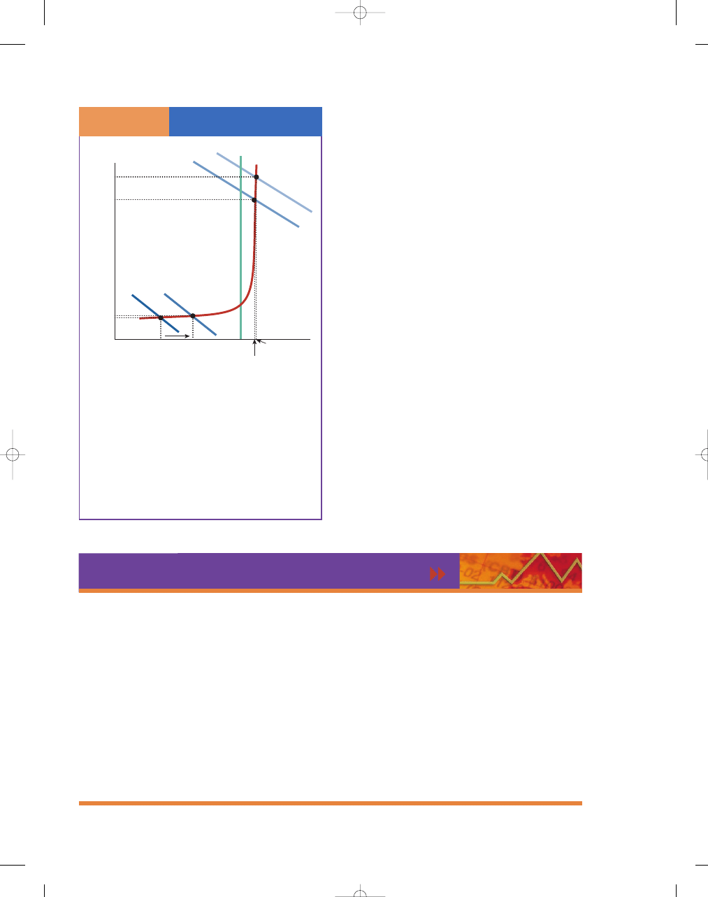
740

M O D U L E 6

Macroeconomic Foundations

Most macroeconomists now believe that price and

wages are not completely inflexible downward.
However, wages and prices do tend to be less flexible
when excess capacity is available—the slope of the
SRAS is flatter the further it is from full employment.
However, when the economy is temporarily operating
beyond RGDP

, the SRAS is steep because higher

output prices are necessary if firms are expanding
output in this unsustainable region beyond full employ-
ment. That is, the firm can increase output by working
labor and capital more intensively. When resources are
idle, output will be responsive to changes in AD, and
the price level will not be as responsive—the SRAS is
flat—the move from AD

to AD

. And when resources

are at full capacity, output is less responsive to changes
in AD and the price level is highly responsive—the
SRAS is steep—the move from AD

to AD

However, economists continue to debate about the

actual shape of the aggregate supply curve.

Although the Keynesian model is helpful in

explaining the events that unfolded in the 1930s, it is
far less useful in explaining today’s economy, an
economy that has seen roughly 2 years of recession in
the past 23 years. In addition, the model fails to
explain the stagflation of the 1970s—unemployment
and inflation together—that is, it does not incorpo-
rate possible shifts in the aggregate supply curve. It
also does not take into consideration the expectations
of consumers and firms as they react to changes in
policies designed to stabilize the economy.

g r e a t e c o n o m i c t h i n k e r s

John Maynard Keynes (1883–1946)

John Maynard Keynes was born in Cambridge, England, in 1883. Keynes’s father
was a political economist and logician, his mother a justice of the peace who
eventually became the mayor of Cambridge, England.

Many would argue that Keynes was one of the most brilliant minds of

the twentieth century. He was educated at Eton and Cambridge, where he
studied mathematics and philosophy. Keynes had a brief tutelage under Alfred
Marshall who tried to convince Keynes to pursue economics. Keynes began his
career in the India Office of the British government. He soon became bored
and returned to King’s College, Cambridge to lecture in economics, a post he
held until his death in 1946.

Keynes had many interests outside of economics, including mathematics,

art, and theater. Keynes married a Russian ballerina and, for a time, he

associated with a group of intellectuals known as Bloomsury Group (which
included such notables as E. M. Forster and Virginia Wolff).

Keynes’s contributions to the field of economics have influenced public

policy since 1930. He is the father of discretionary fiscal policy—deliberating
using government spending and taxes to stabilize the economy.

Keynes believed that the economy could stay in a period of unemploy-

ment for a long time and not self-correct. Specifically, Keynes emphasized the
idea that wages and prices do not always adjust rapid to bring about full
employment in an economy. Keynes believed that government spending could
stimulate the economy back to full employment.

Keynes was also a successful investor in the commodity and stock

markets. His own net worth increased from a miniscule level in 1920 to
over $2 million by the time of his death.

The Keynesian Aggregate
Supply Curve

S E C T I O N

2 6 . 8

X H I B I T

In the flat portion of the SRAS curve, an increase in AD,
from AD

to AD

, has little impact on the price level

but considerable impact on real GDP and employment.
Similarly, a reduction in AD in this region will also leave
the price level relatively unchanged—the price level
does not rise or fall much in this situation, but RGDP
does. When resources are at (or temporarily beyond)
the natural rate, output is not highly responsive to
changes in AD but the price level is responsive—as
shown in the move from AD

to AD

Real GDP, Y

SRAS

LRAS

RGDP

Price Le

vel

95469_26_Ch26_p719-752.qxd 14/1/07 3:01 PM Page 740

C H A P T E R 2 6

The Keynesian Expenditure Model

741

Fill in the blanks:

1. Keynes believed that _____________ was the critical

determinant of the overall level of economic activity.

2. In the simple Keynesian model, we assume that the

price level is _____________ as output changes.

3. _____________ spending is the largest component of

the demand for final goods and services.

4. The _____________ factors affecting consumption are

those that do not depend on income.

5. A(n) _____________ in real wealth would decrease

autonomous consumption.

6. A higher interest rate today tends to make items pur-

chased on credit _____________ expensive and
_____________ expenditures on those items.

7. Either lower interest rates or lower household debt

would tend to _____________ autonomous consumption.

8. An increase in consumer confidence would tend to

_____________ consumption spending.

9. Personal consumption spending depends most impor-

tantly on your current _____________.

10. Your marginal propensity to consume is equal to the

change in _____________ divided by the change in
_____________.

11. The more you spend out of any given increase in income,

the _____________ your marginal propensity to consume.

12. Your marginal propensity to save is equal to the change in

_____________ divided by the change in _____________.

13. The MPC and MPS must add up to _____________.

14. The MPC is equal to the _____________ of the con-

sumption function.

15. Consumption spending is partly _____________, or

independent of income, and partly _____________, or
dependent on income.

16. Income and _____________ are always the same in the

economy.

17. Aggregate _____________ equal _____________ when

the economy is in equilibrium.

18. In the Keynesian model, if output were lower than its

equilibrium level, inventories would _____________
desired levels and producers would _____________
output.

I n t e r a c t i v e S u m m a r y

S E C T I O N

C H E C K

In the most complex form of the Keynesian expenditure model, price level is variable and does impact the compo-

nents of aggregate expenditure due to the real wealth effect, the interest rate effect, and the open economy effect.

The aggregate demand curve is derived by the relationship of the price level and output, plotted by the Keynesian-

cross equilibrium at varying price levels.

Changes in aggregate expenditures for reasons other than price level or output will shift the aggregate demand curve.

When prices are sticky, the SRAS curve is flat, meaning that changes in aggregate demand result in little change in

the price level, but significant changes in RGDP.

Price stickiness is likely when the economy has excess capacity, but is less likely when resources are at full capacity.

In the Keynesian expenditure model, how does a lower price level lead to an increase in the real quantity of goods

and services demanded?

If autonomous expenditures increased by $20 billion, what is the change in aggregate demand at a given price level

if the marginal propensity to consume is 0.75?

If autonomous expenditures decreased by $50 billion, what is the change in aggregate demand at a given price level

if the marginal propensity to consume is 0.8?

Along a vertical long-run aggregate supply curve, what effect will a $10 billion increase in government expenditures

have on real output if the marginal propensity to consume is 0.75? What if the marginal propensity to consume is 0.9?

If the short-run aggregate supply curve is upward sloping, why will the change in real output due to an increase in

autonomous expenditures in the short run be less than that indicated by the multiplier formula?

If wages are sticky downward, why will a decrease in autonomous expenditures reduce real output much like the

Keynesian expenditure model indicates?

95469_26_Ch26_p719-752.qxd 14/1/07 3:01 PM Page 741

742

M O D U L E 6

Macroeconomic Foundations

19. When inventories rise above desired levels, output will

_____________.

20. When aggregate expenditures exceed output, output

will _____________.

21. In addition to consumption, the major components of

aggregate expenditures are _____________,
_____________, and _____________.

22. Only in equilibrium do aggregate expenditures

_____________ output.

23. One reason that investment contributes to the busi-

ness cycle is that _____________ investment responds
dramatically to perceptions about future changes in
business activity.

24. When unplanned inventory investment is

_____________, output will tend to fall.

25. In equilibrium, unplanned business investment

_____________ zero.

26. An increase in autonomous government purchases by

$2 billion will increase output by _____________
$2 billion in the simple Keynesian model.

27. The expenditure multiplier is equal to 1 divided by

_____________, when consumption is the only com-
ponent of aggregate expenditures.

28. When autonomous investment increases, the level of

consumption will _____________ as a result.

29. The _____________ is MPC, the smaller is the expen-

diture multiplier.

30. As well as autonomous consumption, changes in

_____________, _____________, and _____________
can also change autonomous expenditures.

31. When an economy grows rapidly, its imports

_____________, so that its net exports _____________.

32. When components of aggregate expenditures other

than consumption change with income, the multiplier
equals _____________, which is the marginal propen-
sity of aggregate expenditures.

33. MPAE _____________ when the marginal propensity

to consume or the marginal propensity to invest out
of income increases, or the marginal propensity to
import decreases.

34. _____________ taxes are taxes that do not depend on

income.

35. Equilibrium output will tend to move in the

_____________ direction as a change in government
purchases and in the _____________ direction as a
change in lump-sum taxes.

36. The multiplier for changes in lump-sum taxes is

_____________ that for changes in government
purchases.

37. The balanced-budget multiplier is always equal to

_____________.

38. According to the _____________, an autonomous

increase in saving could reduce an economy’s equilib-
rium output.

39. In the Keynesian model, an increase in autonomous

saving yields _____________ benefit to the economy,
but _____________ real output.

40. The government can raise aggregate expenditures

by increasing its spending, but for real output
to increase, something must cause an increase
in _____________.

41. To go from the Keynesian-cross to aggregate demand,

we need to add how the _____________ affects each
of the aggregate expenditure components.

42. Consumption, investment, and net exports all

increase as a result of a _____________ in the
price level.

43. In terms of the Keynesian expenditure model, a fall

in the price level shifts the aggregate expenditures
curve _____________.

44. Changes in any of the components of aggregate

expenditures for any reason other than a change in
the _____________ or _____________ will also shift
the aggregate demand curve.

45. When the aggregate expenditure curve shifts up for

reasons other than changes in the price level, the
aggregate demand curve shifts _____________.

46. The aggregate supply curve must be _____________ in

the long run.

47. If the short-run aggregate supply curve slopes

upward, an increase in aggregate demand will
increase real output _____________ than aggregate
expenditures in the short run.

48. If wages and prices are sticky and the economy has

sufficient excess capacity, the short-run aggregate
supply curve would be _____________ over that range
of output.

49. _____________ and _____________ inflexibility, when

aggregate demand fell, played a significant part in
Keynesian theory.

50. The Keynesian model could not explain the

_____________ of the 1970s.

nswers: 1.

total spending 2.

constant 3.

Consumption 4.

autonomous 5.

decrease 6.

more; reduces 7.

increase 8.

increase

9.disposable income

10.consumption spending; disposable income

11.greater

12.savings; disposable income

13.1

14.slope

15.autonomous; induced

16.output

17.expenditures; output

18.fall below; increase

19.fall

20.rise

21.investment; government

purchases; net exports 22.

equal 23.

planned 24.

positive 25.

equals 26.

more than 27.

−MPC)

28.increase

29.smaller

30.investment; government purchases; net exports

31.rise; fall

32.1/(1

−MP

AE) 33.

increases 34.

Lump-sum 35.

same; opposite

36.less than

37.1

38.paradox of thrift

39.no; reduces

40.aggregate supply

41.price level

42.fall

43.up

44.price level; income

45.right

46.vertical

47.less

48.flat

49.Price; wage

50.stagflation

95469_26_Ch26_p719-752.qxd 14/1/07 3:01 PM Page 742

C H A P T E R 2 6

The Keynesian Expenditure Model

743

autonomous determinants of

consumption expenditures 721

marginal propensity to consume

(MPC) 722

marginal propensity to save (MPS) 723
unplanned inventory investment 728
expenditure multiplier 729

balanced-budget change in fiscal

policy 734

balanced-budget multiplier 734

K e y Te r m s a n d C o n c e p t s

S e c t i o n C h e c k A n s w e r s

26.1 Simple Keynesian Expenditure Model

1. How does the assumption of a fixed price level in the

Keynesian expenditure model solve the problem of
distinguishing between changes in the real value of
a variable (such as GDP) and changes in its nominal
value?

If the price level is fixed, a change in nominal income
is equivalent to a change in real income.

2. Would it be possible for some consumption expendi-

tures to be autonomous and other parts of consump-
tion expenditure not to be autonomous?

Yes. Some consumption depends on income, but
other consumption is autonomous (not changing with
income), depending on variables such as real wealth,
interest rates, etc.

3. In what two ways does a higher interest rate tend to

reduce current consumption?

A higher interest rate reduces current consumption
by (1) increasing the cost of consumption items
bought on credit and (2) increasing the return to cur-
rent saving, which increases savings, which in turn
reduces consumption.

4. What would happen to autonomous consumption

expenditures if the value of a consumer’s stock market
investments rose and his household debt rose at the
same time?

If the value of a consumer’s stock market investments
rose, it would increase autonomous consumption, but
if household debt rose, it would reduce autonomous
consumption. Since these effects are in opposite direc-
tions, the net effect would be indeterminate, without
more information.

5. What would happen to your autonomous consump-

tion if you expected to get a job paying 10 times your
current salary next week?

Since your expected future income will rise substan-
tially, just like an increase in real wealth, it will
increase your current consumption.

6. Why do households headed by a 50-year-old tend to

save a larger fraction of their incomes than those
headed by either a 30-year-old or a 70-year-old?

A 50-year-old is in his peak earning years and is also
trying to save for retirement, both of which increase
saving. A 70-year-old is in retirement and drawing
down previous savings. A 30-year-old has a relatively
low income and is often faced with the expenses of
raising a family.

26.2 Finding Equilibrium in the Keynesian Model

1. If consumption purchases rise with disposable income,

how would an increase in taxes affect consumption
purchases?

An increase in taxes reduces disposable income, which
in turn reduces consumption purchases.

2. If your marginal propensity to consume was 0.75,

what is your marginal propensity to save? If your
marginal propensity to consume rose to 0.80, what
would happen to your marginal propensity to save?

Since the marginal propensity to consume plus the
marginal propensity to save must equal 1, if MPC

0.75, MPS

= 0.25. If MPC = 0.8, MPS = 0.2.

3. Could a student have a positive marginal propensity

to save, and yet have negative savings (increased bor-
rowing) at the same time?

Yes. A student could be increasing his saving (decreasing
his dissaving) with each dollar of income earned, yet
still have an income low enough (less than autonomous
consumption divided by MPS) that he must borrow.

4. What would happen to the slope of the consumption

function if the marginal propensity to save fell?

Since the slope of the consumption function equals
MPC, a fall in MPS implies an increase in MPC and a
steeper consumption function.

5. Why would an increase in disposable income increase

induced consumption but not autonomous consumption?

Autonomous consumption is defined as consumption
spending that does not depend on income, while induced

95469_26_Ch26_p719-752.qxd 14/1/07 3:01 PM Page 743

744

M O D U L E 6

Macroeconomic Foundations

consumption spending is induced by increases in dispos-
able income.

6. What tends to happen to inventories if aggregate

expenditures exceed output? What tends to happen
to output?

If aggregate expenditures exceed output, inventories
will fall, which will give producers incentives to
increase output.

7. What tends to happen to inventories if output exceeds

aggregate expenditures? What tends to happen to
output?

If output exceeds aggregate expenditures, inventories
will rise, giving producers incentives to decrease output.

8. What would equilibrium output be if autonomous

consumption was $2 trillion and the marginal propen-
sity to consume was 0.75?

$2 trillion plus 0.75Y must equal Y, so $2 trillion
equals 0.25Y and Y equals $8 trillion.

9. What would equilibrium output be if autonomous

consumption was $2 trillion and the marginal propen-
sity to consume was 0.80?

$2 trillion plus 0.8Y must equal Y, so $2 trillion
equals 0.2Y and Y equals $10 trillion.

26.3 Adding Investment, Government Purchases,

and Net Exports

1. When all the nonconsumption components of aggre-

gate expenditures are autonomous, why does the
aggregate expenditures line have the same slope as the
consumption function?

The slope of the aggregate expenditures line equals
the change in aggregate expenditures divided by the
change in income, but where only consumption
depends on income, the change in aggregate expendi-
tures equals the change in consumption, and the
aggregate expenditures line has the same slope as the
consumption function.

2. If net exports are negative, what happens to the

aggregate expenditures line, other things equal? What
will happen to equilibrium income?

Autonomous expenditures equals the sum of
autonomous consumption plus investment plus gov-
ernment purchases plus net exports. If net exports are
negative, autonomous expenditures are lower and the
aggregate expenditure line shifts down, resulting in
lower equilibrium income.

3. If autonomous consumption is $2 trillion, invest-

ment purchases plus government purchases plus
net exports is also $2 trillion, and the marginal
propensity to consume is 0.75, what is equilibrium
income?

Autonomous expenditures plus 0.75Y

= Y, so $4 trillion

plus 0.75Y equals Y. Therefore, $4 trillion

= 0.25Y and

= $16 trillion.

4. If autonomous consumption is $2 trillion, invest-

ment purchases plus government purchases plus
net exports is also $2 trillion, and the marginal pro-
pensity to consume is 0.5, what is equilibrium income?

Autonomous expenditures plus 0.8Y = Y, so $4 trillion
plus 0.8Y equals Y. Therefore, $4 trillion

= 0.2Y and

= $20 trillion.

5. As the economy turns toward a recession, what happens

to unplanned inventory investment? Why? What
happens to planned investment? Why?

As the economy turns toward a recession, unplanned
inventory investment is positive because sales are less
than producers’ planned. Planned inventory falls
because it is very sensitive to perceptions of future
changes in business conditions.

6. How does unplanned inventory investment signal

which way real income will tend to change in the
economy?

Unplanned inventory increases signal that demand
was weaker than expected, which will tend to result
in a decrease in real output and income. Unplanned
inventory decreases signal that demand was stronger
than expected, which will tend to result in an increase
in real output and income.

26.4 Shifts in Aggregate Expenditures and the Multiplier

1. If autonomous expenditure rises and the marginal

propensity to consume rises, what would happen to
equilibrium income?

Since equilibrium income equals autonomous expendi-
ture times one divided by one minus MPC, an increase
in autonomous expenditures would increase equilib-
rium income. An increase in MPC would increase the
multiplier, and also increase equilibrium income.

2. If autonomous expenditure rises and the marginal

propensity to consume falls, what would happen to
equilibrium income?

Since equilibriuim income equals autonomous expen-
diture times one divided by one minus MPC, an
increase in autonomous expenditures would increase
equilibrium income. A decrease in MPC would
decrease the multiplier and decrease equilibrium
income. Since the two changes would change equilib-
rium income in opposite directions, we do not know
the net effect without more information.

3. If the marginal propensity to consume was 0.75,

what would happen to equilibrium income if

95469_26_Ch26_p719-752.qxd 14/1/07 3:01 PM Page 744

C H A P T E R 2 6

The Keynesian Expenditure Model

745

government purchases increased by $500 billion
and investment fell by $500 billion at the same
time? What if government purchases increased
by $500 billion and investment fell by $400 billion
at the same time?

If government purchases increased by $500 billion
and investment fell by $500 billion at the same time,
there would be no change in autonomous expenditures
and therefore no change in equilibrium income. If gov-
ernment purchases increased by $500 billion and invest-
ment fell by $400 billion at the same time, autonomous
expenditures would increase by $100 billion. It would
increase equilibrium income by $100 billion times one
over one minus 0.75, or $400 billion.

4. Why does a larger marginal propensity to consume

lead to a larger multiplier?

A larger marginal propensity to consume makes the
denominator of the multiplier smaller, which makes
the multiplier larger.

5. If autonomous consumption was $300 billion, invest-

ment was $200 billion, government purchases were
$400 billion, and net exports were a negative $100
billion, what would autonomous consumption be?
What would equilibrium income be?

Autonomous expenditures are the autonomous com-
ponents of consumption, investment, government pur-
chases plus net exports. Here that would be $300 billion
plus $200 billion plus $400 billion minus $100 billion,
or $800 billion. Equilibrium income would be
$800 billion times one over one minus MPC. We
cannot calculate that number without knowing MPC.

6. What would happen to equilibrium income if, other

things equal, imports increased by $100 billion and
the marginal propensity to consume was 0.9?

Net exports would decrease by $100 billion, which
would decrease autonomous expenditures by
$100 billion. Income would fall by $100 billion times
one over one minus 0.9, or $1 trillion.

26.5 A Complete Model

1. If investment as well as consumption increased with

income, for a given level of autonomous expenditures,
what will happen to equilibrium income?

If investment as well as consumption increased with
income, then MPAE would exceed MPC, and the mul-
tiplier would be larger, resulting in an increase in
equilibrium income.

2. If consumption fell, beginning a recession, but local

government purchases also fell as a result, how would
that affect the resulting change in equilibrium income?

If both consumption and local government purchases
fell, then autonomous expenditures would fall, result-
ing in a lower equilibrium income.

3. What will growth in U.S. income do to net exports?

As U.S. income grows, American purchases also grow.
Some of those purchases come from other countries,
increasing our imports from them, which, in turn,
decreases our net exports.

4. What is MPAE if the marginal propensity to con-

sume was 0.5, the marginal propensity to invest was
0.1, the marginal propensity of government pur-
chases was 0.2, and the marginal propensity to
import was 0.05?

MPAE

= MPC + MPI + MPG − MPM. Here, it is 0.5 +

0.1

+ 0.2 − 0.05, or 0.75.

5. What would happen to the multiplier if the marginal

propensity to consume went up and the marginal
propensity to invest went down at the same time?

If the marginal propensity to consume went up, it
would increase MPAE and increase the multiplier. If
the marginal propensity to invest went down, it
would decrease MPAE and decrease the multiplier.
Since the effects are in opposite directions, the net
effect is indeterminate without more information.

26.6 Government Purchases, Taxes, and

the Balanced-Budget Multiplier

1. If government purchases rise by $10 million and the

marginal propensity to consume is 0.75, what happens
to equilibrium income? If taxes fall by $10 million,
what happens to equilibrium income?

If government purchases rise by $10 million, the
change in Y equals $10 billion times one over one
minus 0.75, or $40 billion. If taxes fall by $10 mil-
lion, the change in equilibrium income equals

−0.75 ×

−$10 billion times one over one minus 0.75, which is
$7.5 billion times 4, or $30 billion.

2. Why will the effect on autonomous consumption of a

given change in taxes equal minus the marginal
propensity to consume times the effect of an equal
change in government purchases?

The change in government purchases is the initial
effect on aggregate demand, which is then multiplied
by the multiplier effect. However, when taxes change,
the initial effect on aggregate demand is not equal to
the change in taxes. It is the change in consumption
spending caused by the change in taxes, which equals
minus MPC times the change in taxes.

3. If a change in equilibrium income was equal to the

change in government purchases that caused it, why
do we know that the government funded the increase
in purchases with an equal increase in taxes?

In this case, the multiplier

= one. However, we know

that the balanced-budget multiplier

= one, so that the

95469_26_Ch26_p719-752.qxd 14/1/07 3:01 PM Page 745

746

M O D U L E 6

Macroeconomic Foundations

government purchases in this case must have been
funded by an equal increase in taxes.

26.7 The Paradox of Thrift

1. Why does an increase in autonomous saving decrease

equilibrium income?

An increase in autonomous saving decreases
autonomous consumption, which decreases autonomous
expenditures, which decreases equilibrium income.

2. If autonomous saving and investment increase by the

same amount, what would be the effect on equilib-
rium income?

If autonomous saving increased, autonomous con-
sumption would decrease the same amount.
Therefore, autonomous consumption would decrease
the same amount as investment increased, and there
would be no net effect on autonomous expenditures,
and so no net effect on equilibrium income.

3. If autonomous expenditures were $1 trillion and the

marginal propensity to save increased from 0.20 to
0.25, what would happen to equilibrium income?

Initially, equilibrium income would be $1 trillion times
one divided by 0.20, or $5 trillion. If MPS changed to
0.25, equilibrium income would be $1 trillion times
one divided by 0.25, or $4 trillion.

4. Why is the Keynesian expenditure model’s assumption

of a fixed price level misleading once the productive
capacity of the economy is reached?

Real output is inherently limited by scarce resources.
An increase in aggregate expenditures cannot increase
real output beyond an economy’s productive capacity.

26.8 Keynesian-Cross to Aggregate Demand

1. In the Keynesian expenditure model, how does a

lower price level lead to an increase in the real quan-
tity of goods and services demanded?

A lower price level increases real consumption due to
the real balance effect, increases investment because
of the interest rate effect, and increases net exports,
all of which increase the real quantity of goods and
services demanded.

2. If autonomous expenditures increased by $20 billion,

what is the change in aggregate demand at a given price
level if the marginal propensity to consume is 0.75?

AD would increase by the increase in autonomous
expenditures times one over one minus MPC, or
$20 billion

× 4 = $80 billion.

3. If autonomous expenditures decreased by $50 billion,

what is the change in aggregate demand at a given price
level if the marginal propensity to consume is 0.8?

AD would decrease by the decrease in autonomous
expenditures times one over one minus MPC, or
$50 billion

× 5 = $250 billion.

4. Along a vertical long-run aggregate supply curve,

what effect will a $10 billion increase in government
expenditures have on real output if the marginal
propensity to consume is 0.75? What if the marginal
propensity to consume is 0.9?

A change in aggregate expenditures, increasing aggregate
demand, will have no effect on real output along a verti-
cal long-run aggregate supply curve, regardless of MPC.

5. If the short-run aggregate supply curve is upward

sloping, why will the change in real output due to
an increase in autonomous expenditures in the
short run be less than that indicated by the multi-
plier formula?

The multiplier indicates how far right the AD curve will
shift, which is how much real output would increase if
the short-run aggregate supply curve was horizontal.
However, since the short-run aggregate supply curve is
upward sloping, real output will increase less than the
amount indicated by the multiplier formula.

6. If wages are sticky downward, why will a decrease in

autonomous expenditures reduce real output much
like the Keynesian expenditure model indicates?

A decrease in autonomous expenditures will reduce
AD by the amount indicated by the multiplier for-
mula. If wages are sticky downward, the short-run
aggregate supply curve will be nearly horizontal over
the relevant range, and the fall in real output would
be nearly as great as the fall in AD.

95469_26_Ch26_p719-752.qxd 14/1/07 3:01 PM Page 746

H A P T E R

2 6

S T U D Y

G U I D E

747

True or False

1. In the Keynesian model, when total spending increases, firms increase their output and hire more workers.

2. When we assume the price level is constant, we do not have to distinguish real variable changes from nominal variable

changes.

3. The Keynesian approach assumes that prices and wages were constant until we reach full employment.

4. Disposable income is one of the dominant factors in determining the demand for consumer goods.

5. An increase in property values or a stock market boom would tend to reduce autonomous consumption.

6. If either interest rates fell or the level of household debt rose, autonomous consumption would tend to fall.

7. A decrease in consumer confidence would tend to reduce consumption spending.

8. Consumption spending depends most importantly on people’s expected future disposable income.

9. If your disposable income increased by $10,000 and as a result, your consumption spending increased by $8,000,

you would have a marginal propensity to consume of 0.8.

10. The higher is MPC, the lower is MPS.

11. If your MPC was equal to 0.5, your MPS would also be 0.5.

12. The greater is the MPS, the steeper is the slope of the consumption function.

13. When your disposable income rises, both your total consumption and your total saving rise.

14. Aggregate expenditures always equal consumption expenditures.

15. Income equals output in the economy only in equilibrium.

16. When output is greater than the equilibrium level, inventories would build up above desired levels and producers

would reduce output.

17. In the Keynesian model, when inventories fall below desired levels, output will rise.

18. When output is less than aggregate expenditures, output will fall.

19. The greater is savings, for a given level of income, the greater is aggregate expenditures.

20. If investment, government purchases, and net exports are autonomous, the aggregate expenditures curve will have the

same slope as the consumption function.

21. Planned investment is sensitive to firms’ perceptions about the future.

22. If businesspeople are confident that the economy will be good in the future, output tends to increase.

23. When unplanned inventory investment is negative, output will tend to fall.

24. Increasing planned investment would tend to increase output, but positive unplanned inventory investment would

tend to decrease output.

25. The expenditure multiplier applies to any increase in autonomous expenditures.

26. An increase of $10 million in autonomous consumption has the same effect on output as $10 million increase in

autonomous investment.

27. The multiplier process takes place almost instantaneously.

28. Whenever a component of autonomous expenditures increases, consumption will tend to increase as a result.

29. The greater is MPC, the greater is the expenditure multiplier.

30. If MPC equals 0.75, the expenditure multiplier equals 4.

31. Investment as well as consumption spending can depend on current income.

32. MPAE equals MPC, plus the marginal propensity to invest out of income, plus the marginal propensity of govern-

ment spending out of income, minus the marginal propensity to import.

33. If the marginal propensity to invest out of income and the marginal propensity to import both increase, MPAE would

increase.

34. If the marginal propensity to import equaled zero, MPAE would equal MPC.

747

S T U D Y

G U I D E

95469_26_Ch26_p719-752.qxd 14/1/07 3:01 PM Page 747

35. When lump-sum taxes rise, consumers will decrease autonomous consumption spending by the change in lump-sum

taxes times the MPC.

36. A $1 billion increase in government purchases will have a greater effect on equilibrium output than a $1 billion

decrease in lump-sum taxes.

37. The greater is MPC, the greater is the balanced-budget multiplier.

38. If government purchases increased by $10 billion and lump-sum taxes decreased by $10 billion, equilibrium output

will increase by $10 billion.

39. An autonomous increase in saving would also be a decrease in autonomous consumption, resulting in decreased

output, in the Keynesian model.

40. The paradox of thrift is that even though thrift is desirable for an individual, it might cause problems for the econ-

omy as a whole, in the Keynesian model.

41. What is missing in the Keynesian expenditure model is the notion of supply.

42. The Keynesian expenditure model is best seen as a model of aggregate demand, and not a complete model of the economy.

43. The components of aggregate demand depend on the price level.

44. An increase in the price level would increase investment but decrease net exports.

45. An increase in the price level shifts up the aggregate expenditure function.

46. A change in the price level would shift the aggregate expenditure function but not aggregate demand.

47. When the aggregate expenditures function shifts up because of an increase in autonomous expenditures due to

increased optimism, aggregate demand will shift right.

48. The price level has no effect on real output in the long run.

49. In the long run, an increase in government purchases will increase aggregate demand but not real output.

50. In the short run, an increase in aggregate demand will increase real output by an amount equal to the change in

government purchases multiplied by 1/(1

− MPC).

51. The expenditure multiplier tells how much an increase in autonomous expenditures will increase real output in the

short run and in the long run.

52. On the flat part of a short-run aggregate supply curve, a decrease in aggregate demand will decrease real output and

not change the price level.

53. In the simple Keynesian model, the price level cannot increase as real output falls.

Multiple Choice

1. Demand for consumer goods will be affected by which of the following?

a. disposable income
b. credit conditions
c. the level of debt outstanding
d. expectations about the future
e. all of the above

2. Autonomous consumption will increase when

a. real wealth increases.
b. the interest rate increases.
c. household debt increases.
d. any of the above occur.

3. If autonomous consumption fell, it could have been caused by

a. falling interest rates.
b. falling household debt.
c. more optimistic expectations about future disposable income.
d. increasing real wealth.
e. none of the above.

748

95469_26_Ch26_p719-752.qxd 14/1/07 3:01 PM Page 748

4. If an economy’s marginal propensity to consume was 0.75, which of the following is not true?

a. The consumption function would have a slope of 0.75.
b. The marginal propensity to save would be 0.25.
c. Increases in disposable income would increase consumption spending by three times as much as it

would increase saving.

d. Consumption will always equal 75 percent of disposable income.
e. All of the above would be true.

5. Which of the following need not be equal at equilibrium in the Keynesian model?

a. income and output
b. aggregate expenditures and output
c. consumption and income
d. All of the above must be equal at equilibrium in the Keynesian model.

6. If output was lower than its equilibrium level,

a. inventories will exceed their desired level.
b. output will rise.
c. total expenditures will fall.
d. the marginal propensity to consume will rise.

7. Output equals income

a. always.
b. only in equilibrium.
c. only when MPC equals MPS.
d. unless inventories are changing.

8. In addition to consumption, the major components of aggregate expenditures do not include

a. investment.
b. saving.
c. government purchases.
d. net exports.
e. All of the above are included in aggregate expenditures.

9. When the autonomous level of investment increases,

a. at first, inventories will fall below desired levels.
b. output will rise.
c. consumption spending will rise.
d. all of the above will occur.

10. Equilibrium output will tend to increase when

a. planned investment increases.
b. unplanned investment is positive.
c. either planned investment increases or unplanned investment is positive.
d. either planned investment decreases or unplanned investment is negative.

11. Which of the following would increase aggregate expenditures?

a. Households become more optimistic about the future.
b. Interest rates fall.
c. Foreign economies improve.
d. Government purchases increase.
e. Any of the above would increase aggregate expenditures.

12. Which is true regarding the expenditure multiplier?

a. It is defined as 1/MPC.
b. Its effects take place almost instantaneously.
c. The higher the MPC, the greater the expenditure multiplier.

749

95469_26_Ch26_p719-752.qxd 14/1/07 3:01 PM Page 749

d. All of the above are true.
e. None of the above is true.

13. Equilibrium output would tend to rise when

a. autonomous expenditures increase.
b. the MPC increases.
c. either autonomous expenditures increase or the MPC increases.
d. neither autonomous expenditures increase nor the MPC increases.

14. If the MPC equals 0.5,

a. the expenditure multiplier will equal 2.
b. a $5 billion increase in investment would tend to increase output by $10 billion.
c. the expenditure multiplier is less than if the MPC

= 0.8.

d. all of the above are true.

15. Investment can depend on

a. expectations.
b. taxes.
c. interest rates.
d. current income.
e. all of the above.

16. Which of the following is negatively related to income?

a. net exports
b. government purchases
c. investment
d. consumption
e. None of the above is negatively related to income.

17. Which of the following would tend to decrease the marginal propensity of aggregate expenditure?

a. an increase in the marginal propensity to consume
b. an increase in the marginal propensity to invest
c. an increase in the marginal propensity of government purchases
d. an increase in the marginal propensity to import
e. None of the above would tend to decrease the marginal propensity of aggregate expenditure.

18. The expenditure multiplier would tend to increase whenever

a. the marginal propensity to invest increased.
b. the marginal propensity to consume decreased.
c. the marginal propensity of government purchases decreased.
d. the marginal propensity to consume increased.
e. either a or d occurs.

19. If the MPC equaled 0.75, a $100 billion decrease in lump-sum taxes would

a. increase output by $75 billion.
b. increase output by $100 billion.
c. increase output by $300 billion.
d. increase output by $400 billion.
e. do none of the above.

20. If the MPC equaled 0.75, a $100 billion increase in government purchases, combined with a $100 billion

increase in lump-sum taxes, would

a. increase output by $100 billion.
b. increase output by $300 billion.
c. increase output by $400 billion.
d. increase output by $700 billion.

750

95469_26_Ch26_p719-752.qxd 14/1/07 3:02 PM Page 750

21. If the MPC equaled 0.75, a $100 billion increase in government purchases, combined with a $100 billion

decrease in lump-sum taxes, would

a. increase output by $100 billion.
b. increase output by $300 billion.
c. increase output by $400 billion.
d. increase output by $700 billion.

22. Which of the following multipliers is greatest?

a. the balanced-budget multiplier
b. the government purchases multiplier
c. the tax multiplier
d. They are all the same.

23. When the price level falls,

a. consumption increases because real wealth increases.
b. investment rises because interest rates decline.
c. net exports rise because exchange rates decline.
d. all of the above are true.

24. Which of the following would shift both the aggregate expenditures function and aggregate demand?

a. an increase in consumption because disposable income rose
b. an increase in consumption because the price level fell
c. an increase in consumption because of increased consumer optimism
d. All of the above would shift both the aggregate expenditures function and aggregate demand.

25. The expenditure multiplier tells how much

a. aggregate demand shifts when autonomous expenditures change.
b. real output increases in the short run when autonomous expenditures change.
c. real output increases in the long run when autonomous expenditures change.
d. real output changes in the short run when autonomous expenditures change.

26. If the economy was operating on the flat segment of the short-run aggregate supply curve, an increase in

aggregate demand would

a. increase output and increase the price level.
b. increase output and decrease the price level.
c. decrease output and increase the price level.
d. decrease output and decrease the price level.
e. do none of the above.

Problems

1. Which of the following are likely to cause a reduction in consumption?

a. an increase in interest rates
b. an increase in the value of stock market portfolios
c. a decrease in disposable income
d. an increase in income taxes
e. deflation

2. Identify the most volatile component of aggregate expenditure. Identify its largest component.

3. Which of the following will cause the aggregate expenditure schedule to increase?

a. an increase in consumer optimism
b. an increase in the purchase of imports
c. an increase in the sale of exports
d. pessimism by business owners about the outlook of the economy
e. an increase in government spending due to the outbreak of war

751

95469_26_Ch26_p719-752.qxd 14/1/07 3:02 PM Page 751

4. Consumption equals $32,000 when disposable income equals $40,000. Consumption increases to $38,000 when dis-

posable income increases to $50,000. What is the marginal propensity to consume? The marginal propensity to save?
What is the value of the spending multiplier?

5. Calculate equilibrium output when autonomous consumption equals $2 trillion, the MPC equals 0.8, investment

equals $400 billion, government spending equals $800 billion, and net exports equal

−$100 billion.

6. What happens to inventory levels when real output equals $5 trillion, consumption equals $3.5 trillion, planned

investment equals $400 billion, government spending equals $1.3 trillion, and net exports equal $250 billion? What
can you predict will happen to planned production as a result?

7. If the government reduces spending by $75 billion and cuts taxes by an equal amount, predict the impact on overall

output in the economy.

8. Real output equals $7 trillion, consumption equals $4 trillion, planned investment equals $500 billion, government

spending equals $2.4 trillion, and net exports equal

−$200 billion. Is the economy in equilibrium? Why or why not?

If not, predict whether production will increase or decrease.

9. Evaluate the following statement: The Keynesian assumption of wage and price rigidity best corresponds to the steepest

portion of the aggregate supply curve where factories are operating below capacity.

10. Visit the Economy at a Glance page at the Bureau of Economic Analysis, http://www.bea.gov/bea/glance.htm. Locate

information about recent changes in inventory levels as well as the ratio of inventory to sales. Can you detect a trend
upward or downward in inventory levels? What does the trend bode for national output according to the Keynesian-
cross model?

11. Calculate the expenditure multipliers that would exist for the following marginal propensities to consume:

a. 0.95
b. 0.90
c. 0.80
d. 0.75
e. 0.60
f.

0.50

12. Calculate what change in output would result from each of the following circumstances:

a. Autonomous expenditures increase by $40,000 and MPC

= 0.95.

b. Autonomous expenditures increase by $80,000 and MPC

= 0.90.

c. Autonomous expenditures increase by $160,000 and MPC

= 0.80.

d. Autonomous expenditures increase by $200,000 and MPC

= 0.75.

13. What would the multiplier be if

a. MPC

= 0.60.

b. MPC

= 0.60; MPI = 0.10; MPG = 0.10; MP import = 0.05.

c. MPC

= 0.80.

d. MPC

= 0.80; MPI = 0.02; MPG = 0.03; MP import = 0.10.

752

95469_26_Ch26_p719-752.qxd 14/1/07 3:02 PM Page 752

C H A P T E R 2 7

Fiscal Policy

755

Section 27.1 Fiscal Policy 756

Global Watch

Japan’s Fiscal Policy Experiment 757

Section 27.2 Fiscal Policy and the AD/AS Model 758

In the News

The 2003 Tax Cut 759

Global Watch

Global Tax Comparisons: Tax Revenues as a

Percentage of GDP 760

Policy Application

The New Deal and Expansionary

Fiscal Policy? 760

Section 27.3 The Multiplier Effect 761

In the News

Boeing Multiple-Use Fighter Jet Completes

Flight: Developmental Aircraft in Race for Huge
Contract 764

Using What You’ve Learned

The Broken Window

Fallacy 765

Section 27.4 Supply-Side Effects of Tax Cuts 766

Policy Application

Fiscal Policy in its Prime, the 1960s 769

Section 27.5 Automatic Stabilizers 770

Section 27.6 Possible Obstacles to Effective Fiscal

Policy 771

Section 27.7 The National Debt 773

Policy Application

Would a Balanced Budget

Amendment Work? 776

Study Guide

Chapter 27 783

C H A P T E R 2 8

Monetary Institutions

791

Section 28.1 What Is Money? 792

In the News

Tiny Micronesian Island Uses Giant Stones as

Currency 793

Section 28.2 Measuring Money 795

Using What You’ve Learned

Pawn Shops and Liquidity 799

Section 28.3 How Banks Create Money 800

Section 28.4 The Money Multiplier 806

Section 28.5 The Collapse of America’s Banking System,

1920–1933 808

Study Guide

Chapter 28 815

C H A P T E R 2 9

The Federal Reserve System and

Monetary Policy

821

Section 29.1 The Federal Reserve System 822

Section 29.2 The Equation of Exchange 825

Section 29.3 Implementing Monetary Policy: Tools

of the Fed 827

Using What You’ve Learned

Open Market Operations 828

Section 29.4 Money, Interest Rates, and Aggregate

Demand 831

Section 29.5 Expansionary and Contractionary Monetary

Policy 838

In the News

The U.S. Economy in the Wake of

September 11 839

Using What You’ve Learned

Money and the AD/AS

Model 841

In the News

The Science (and Art) of Monetary Policy 842

Great Economic Thinkers

Milton Friedman (1912–2006) 843

Section 29.6 Problems in Implementing Monetary and

Fiscal Policy 843

In the News

Fed Chief Sees Decline Over: House Passes

Recovery Bill 846

Study Guide

Chapter 29 855

C H A P T E R 3 0

Issues in Macroeconomic Theory

and Policy

865

Section 30.1 The Phillips Curve 866

Section 30.2 The Phillips Curve over Time 868

Section 30.3 Rational Expectations and Real

Business Cycles 873

Section 30.4 Controversies in Macroeconomic Policy 878

Study Guide

Chapter 30 887

M O D U L E

O N E T A R Y A N D

I S C A L

O L I C Y

95469_27_ch27_p753-790.qxd 17/1/07 4:06 PM Page 753

95469_27_ch27_p753-790.qxd 5/1/07 10:17 AM Page 754