
13
C H A P T E R
F
I R M S I N
P
E R F E C T L Y
C
O M P E T I T I V E
M
A R K E T S
13.1
The Four Market Structures
13.2An Individual Price Taker's
Demand Curve
13.3
Profit Maximization
13.4 Short-Run Profits and Losses
13.5 Long-Run Equilibrium
13.6 Long-Run Supply
n the previous chapter we discussed the costs of
production. In this chapter, we put the cost of
production together with demand and the mar-
ginal analysis we learned in earlier chapters to
see how a firm must answer two critical questions:
What price should we charge for the goods and
services we sell, and how much should we pro-
duce? The answers to these two questions will
depend on the market structure.
The behavior of firms will depend on the
number of firms in the market, the ease with which
firms can enter and exit the market, and the ability
of firms to differentiate their products from those
of other firms. There is no typical industry. An
industry might include one firm that dominates the
market, or it might consist of thousands of smaller
firms that each produce a small fraction of the
market supply. Between these two end points are
many other industries. However, because we cannot
examine each industry individually, we break them
into four main categories: perfect competition,
monopoly, monopolistic competition, and oligopoly.
In a perfectly competitive market, the market
price is the critical piece of information that a firm
needs to know, a firm in a perfectly competitive
market can sell all it wants at the market price. A
firm in a perfectly competitive market is said to be
a price taker, because it cannot appreciably affect
the market price for its output or the market price
for its inputs. For example, suppose a Washington
apple grower decides that he wants to get out of
the family business and go to work for Microsoft.
Because he may be one of 50,000 apple growers in
the United States, his decision will not appreciably
change the price of the apples, the production of
apples, or the price of inputs.
■
I
F
I R M S I N
P
E R F E C T L Y
C
O M P E T I T I V E
M
A R K E T S
95469_13_Ch13_p331-364.qxd 29/12/06 12:40 PM Page 331

332
M O D U L E 3
Households, Firms, and Market Structure
Economists have identified four market structures in
which firms operate: perfect competition, monopolistic
competition, oligopoly, and monopoly. Certain key
characteristics distinguish each structure or environ-
ment from the other structures. In practice, it is some-
times difficult to decide precisely which structure a given
firm or industry most appropriately fits, because the
dividing line between the structures is not crystal clear.
In the next few paragraphs, we will briefly summarize
the major characteristics of each market structure.
PERFECT COMPETITION
A competitive market is a market situation character-
ized by a large number of buyers and sellers. Firms in
a
perfectly competitive market
sell homogeneous
or standardized products like wheat or apples. New
firms can easily enter the market.
MONOPOLISTIC COMPETITION
Monopolistic competition
falls between perfect
competition and monopoly. Monopolistic competi-
tion is a market struc-
ture in which firms
have both an element
of competition and an
element of monopoly
power. In this market
structure, there are a
relatively large number
of sellers producing dif-
ferentiated products
(restaurants, meals,
cloths, books). There is
considerable non price
competition as firms try to distinguish their product
from others. In this market structure, entry and exit is
very easy.
OLIGOPOLY
Oligopoly
exists when a few firms produce similar
or identical goods. The oligopolist is very con-
scious of the actions of competing firms. Oligopoly
may involve a stan-
dardized product (such
as steel, aluminum, or
crude oil) or a differ-
entiated one (such as
automobiles, breakfast
cereals, refrigerators,
or TVs).
MONOPOLY
At the other end of the continuum of market environ-
ments is
monopoly.
In this market structure, one firm
produces a good or
service that has no close
substitutes, and poten-
tial entrants into the
market must overcome
significant barriers. The
monopolists’ product is
unique, there are no close substitutes. Examples of
monopoly include public utilities (electric, water, and
natural gas suppliers) and first class mail delivery by
the U.S. Postal Service.
Economists often distinguish the perfectly com-
petitive market from the imperfectly competitive
markets of monopolistic competition, oligopoly, and
monopoly. The differences between these markets
will become clearer as we look at them separately in
the chapters to come. Because we will often compare
perfect competition to the other market structures,
let us start by taking a closer look at perfectly com-
petitive markets.
Exhibit 1 summarizes the characteristics of the
four market structures in which firms operate: per-
fect competition, monopolistic competition, oligop-
oly, and monopoly. Each structure or environment
has certain key characteristics that distinguish it from
the other structures. In practice, it is sometimes diffi-
cult to decide precisely which structure a given firm
or industry most appropriately fits, because the
dividing line between the structures is not always
crystal clear.
S E C T I O N
13.1
T h e F o u r M a r k e t S t r u c t u r e s
■
What are the four market structures?
■
What are the characteristics of a firm in a
perfectly competitive market?
■
What is a price taker?
oligopoly
a market structure with only a few
sellers offering similar or identical
products
monopoly
the single supplier of a product
that has no close substitute
perfectly competitive
market
a market with many buyers and sell-
ers selling homogeneous goods, easy
market entry and exit, and no firm
able to affect the market price
monopolistic
competition
a market structure with many firms
selling differentiated products
95469_13_Ch13_p331-364.qxd 29/12/06 12:40 PM Page 332

C H A P T E R 1 3
Firms in Perfectly Competitive Markets
333
A PERFECTLY COMPETITIVE MARKET
This chapter examines perfect competition, a market
structure characterized by (1) many buyers and sellers,
(2) identical (homogeneous) products, and (3) easy
market entry and exit. Let’s examine these characteris-
tics in greater detail.
Many Buyers and Sellers
In a perfectly competitive market, there are many
buyers and sellers; perhaps thousands or conceivably
millions. Because each firm is so small in relation to
the industry, its production decisions have no impact
on the market—each regards price as something over
which it has little control. For this reason, perfectly
competitive firms are called price takers: They must
take the price given by the market because their
influence on price is insignificant. If the price of
apples in the apple market is $2 a pound, then indi-
vidual apple farmers will receive $2 a pound for their
apples. Similarly, no single buyer of apples can
influence the price of apples, because each buyer pur-
chases only a small amount of the apples traded. We
will see how this relationship works in more detail in
Section 13.2.
Identical (Homogeneous) Products
Consumers believe that all firms in perfectly competi-
tive markets sell identical (or homogeneous) products.
For example, in the wheat market, it is not possible to
determine any significant and consistent qualitative
differences in the wheat produced by different farm-
ers. Wheat produced by Farmer Jones looks, feels,
smells, and tastes like that produced by Farmer Smith.
In short, a bushel of wheat is a bushel of wheat. The
products of all the firms are considered to be perfect
substitutes.
Easy Entry and Exit
Product markets characterized by perfect competi-
tion have no significant barriers to entry or exit.
Therefore it is fairly easy for entrepreneurs to
become suppliers of the product or, if they are
already producers, to stop supplying the product.
“Fairly easy” does not mean that any person on the
street can instantly enter the business but rather that
the financial, legal, educational, and other barriers to
entering the business are modest, enabling large
numbers of people to overcome the barriers and
enter the business if they so desire in any given
Can the owner of this orchard charge a noticeably higher
price for apples of similar quality to those sold at the orchard
down the road? What if she charges a lower price for apples
of similar quality? How many apples can she sell at the
market price?
©
Photodisc Green/Getty Images
Perfect
Monopolistic
Characteristic
Competition
Competition
Oligopoly
Monopoly
Number of firms
Very many
Many
A few
One
Barriers to entry or
No substantial ones
Minor barriers
Considerable barriers
Extremely great
exit from industry
Type of product
Homogeneous
Differentiated
Homogeneous or
Unique, no close
differentiated
substitute
Key characteristic
Firms are price takers
Product differentiation
Mutual
Only one firm
interdependence
Examples
Agriculture
Retail trade, restaurants
Steel, automobiles,
Local utilities
household appliances
Characteristics of the Four Major Market Structures
S E C T I O N
1 3 .1
E
X H I B I T
1
95469_13_Ch13_p331-364.qxd 29/12/06 12:40 PM Page 333

334
M O D U L E 3
Households, Firms, and Market Structure
period. If buyers can easily switch from one seller to
another and sellers can easily enter or exit the indus-
try, then they have met the perfectly competitive con-
dition of easy entry and exit. Because of this easy
market entry, perfectly competitive markets generally
consist of a large number of small suppliers.
A perfectly competitive market is approximated
most closely in highly organized markets for securities
and agricultural commodities, such as the New York
Stock Exchange or the Chicago Board of Trade. Wheat,
corn, soybeans, cotton, and many other agricultural
products are sold in perfectly competitive markets.
Although all the criteria for a perfectly competitive
market are rarely met, a number of markets come close
to satisfying them. Even when all the assumptions don’t
hold, it is important to note that studying the model of
perfect competition is useful because many markets
resemble perfect competition—that is, markets in
which firms face highly elastic (flat) demand curves and
relatively easy entry and exit. The model also gives us
a standard of comparison. In other words, we can
make comparisons with the perfectly competitive
model to help us evaluate what is going on in the real
world.
At the Chicago Board of Trade (CBOT), prices are set by thou-
sands of buyers interacting with thousands of sellers. The
goods in question are typically standardized (e.g., grade A
winter wheat), and information is readily available. Every
buyer and seller in the market knows the price, the quantity,
and the quality of the wheat. Transaction costs are negligible.
For example, if a news story breaks on an infestation in the
cotton crop, the price of cotton will rise immediately. CBOT
price information is used to determine the value of a particu-
lar commodity all over the world.
©
Cour
tesy of the Chicago Board of
T
rade
S E C T I O N
*
C H E C K
1.
The four main market structures are perfect competition, monopolistic competition, oligopoly, and
monopoly.
2.
A perfectly competitive market is characterized by many buyers and sellers, an identical (homogeneous)
product, and easy market entry and exit.
3.
Consumers believe that all firms in perfectly competitive markets sell virtually identical (homogeneous)
products. The products of all firms are considered to be perfect substitutes.
4.
In markets with so many buyers and so many sellers, neither buyers nor sellers have any control over price in
perfect competition. They must take the going price and hence are called price takers.
5.
Firms in a perfectly competitive markets have no significant barriers to entry. That is, the barriers are
significantly modest, so that many sellers can enter or exit the industry.
1.
Why do firms in perfectly competitive markets involve homogeneous goods?
2.
Why does the absence of significant barriers to entry tend to result in a large number of suppliers?
3.
Why does the fact that perfectly competitive firms are small relative to the market make them price
takers?
4.
Why is the market for used furniture unlikely to be perfectly competitive?
5.
How is pure monopoly the opposite of perfect competition?
95469_13_Ch13_p331-364.qxd 29/12/06 12:41 PM Page 334

C H A P T E R 1 3
Firms in Perfectly Competitive Markets
335
AN INDIVIDUAL FIRM’S DEMAND CURVE
Perfectly competitive firms are
price takers;
that is,
they must sell at the market-determined price, where
the market price and
output are determined
by the intersection of
the market supply and
demand curves, as seen
in Exhibit 1(b).
Individual wheat farm-
ers know that they
cannot dispose of their wheat at any figure higher than
the current market price; if they attempt to charge a
higher price, potential buyers will simply make their
purchases from other wheat farmers. Further, the farm-
ers certainly would not knowingly charge a lower price,
because they could sell all they want at the market price.
Likewise, in a perfectly competitive market,
individual sellers can change their outputs, and it
will not alter the market price. The large number of
sellers who are selling identical products make this
situation possible. Each producer provides such a
small fraction of the total supply that a change in the
amount he offers does not have a noticeable effect
on market equilibrium price. In a perfectly competi-
tive market, then, an individual firm can sell as much
as it wishes to place on the market at the prevailing
price; the demand, as seen by the seller, is perfectly
elastic.
It is easy to construct the demand curve for an
individual seller in a perfectly competitive market.
Remember, she won’t charge more than the market
price because no one will buy it, and she won’t
charge less because she can sell all she wants at the
market price. Thus, the farmer’s demand curve is
S E C T I O N
13.2
A n I n d i v i d u a l P r i c e Ta k e r ’s
D e m a n d C u r v e
■
Why won’t individual price takers raise or
lower their prices?
■
Can individual price takers sell all they
want at the market price?
■
Will the position of individual price takers’
demand curves change when market price
changes?
Market and Individual Firm Demand Curves in a Perfectly Competitive Market
S E C T I O N
1 3 . 2
E
X H I B I T
1
Price
100
200
d
Quantity of Wheat
(bushels)
0
$5
Firm's Demand
Curve
Firm is a price taker
—must take market price
150
D
S
Quantity of Wheat
(millions of bushels)
0
$5
Market price
and output
determined
here
At the market price for wheat, $5, the individual farmer can sell all the wheat he wishes. Because each producer
provides only a small fraction of industry output, any additional output will have an insignificant impact on market
price. The firm’s demand curve is perfectly elastic at the market price.
a. Individual Firm Demand Curve
b. Market Supply and Demand Curve
price takers
a perfectly competitive firm that
takes the price it is given by the
intersection of the market demand
and market supply curves
95469_13_Ch13_p331-364.qxd 29/12/06 12:41 PM Page 335

336
M O D U L E 3
Households, Firms, and Market Structure
horizontal over the entire range of output that she
could possibly produce. If the prevailing market
price of the product is $5, the farmer’s demand
curve will be represented graphically by a horizon-
tal line at the market price of $5, as shown in
Exhibit 1(a).
A CHANGE IN MARKET PRICE AND
THE FIRM’S DEMAND CURVE
To say that producers under perfect competition
regard price as a given is not to say that price is con-
stant. The position of the firm’s demand curve varies
with every change in the market price. In Exhibit 2,
we see that when the market price for wheat
increases, say as a result of an increase in market
demand, the price-taking firm will receive a higher
price for all its output. Or when the market price
decreases, say as a result of a decrease in market
demand, the price-taking firm will receive a lower
price for all its output.
In effect, sellers are provided with current infor-
mation about market demand and supply conditions
as a result of price changes. It is an essential aspect of
the perfectly competitive model that sellers respond
to the signals provided by such price movements, so
they must alter their behavior over time in the light
of actual experience, revising their production deci-
sions to reflect changes in market price. In this
respect, the perfectly competitive model is straight-
forward; it does not assume any knowledge on the
part of individual buyers and sellers about market
demand and supply—they only have to know the
price of the good they sell.
Market Prices and the Position of a Firm’s Demand Curve
S E C T I O N
1 3 . 2
E
X H I B I T
2
Quantity
(market)
0
$5
$6
Q
1
Q
2
D
2
S
D
1
d
1
d
2
Price
Quantity
(firm)
0
$5
$6
The position of the firm’s demand curve will vary with every change in the market price.
S E C T I O N
*
C H E C K
1.
An individual seller won’t sell at a higher price than the going price, because buyers can purchase the same good
from someone else at the going price.
2.
Individual sellers won’t sell for less than the going price, because they are so small relative to the market that they
can sell all they want at the going price.
3.
The position of the individual firm’s demand curve varies directly with the market price.
1.
Why would a perfectly competitive firm not try to raise or lower its price?
2.
Why can we represent the demand curve of a perfectly competitive firm as perfectly elastic (horizontal) at the
market price?
3.
How does an individual perfectly competitive firm’s demand curve change when the market price changes?
4.
If the marginal cost facing every producer of a product shifted upward, would the position of a perfectly competi-
tive firm’s demand curve be likely to change as a result? Why or why not?
95469_13_Ch13_p331-364.qxd 29/12/06 12:41 PM Page 336

C H A P T E R 1 3
Firms in Perfectly Competitive Markets
337
REVENUES IN A PERFECTLY COMPETITIVE MARKET
The objective of the firm is to maximize profits. To
maximize profits, the firm wants to produce the
amount that maximizes the difference between its
total revenues and total costs. In this section, we will
examine the different ways to look at revenue in a
perfectly competitive market: total revenue, average
revenue, and marginal revenue.
TOTAL REVENUE
Total revenue (TR)
is the revenue that the firm
receives from the sale of its products. Total revenue
from a product equals
the price of the good (P)
times the quantity (q) of
units sold (TR
P
q). For example, if a
farmer sells 10 bushels
of wheat a day for $5 a
bushel, his total revenue is $50 ($5
10 bushels).
(Note: We will use the lowercase letter q to denote
the single firm’s output and reserve the uppercase
letter Q for the output of the entire market. For
example, q would be used to represent the output of
one lettuce grower, while Q would be used to repre-
sent the output of all lettuce growers in the lettuce
market.)
AVERAGE REVENUE AND MARGINAL REVENUE
Average revenue (AR)
equals total revenue divided by
the number of units sold of the product (TR
q, or
[P
q] q). For
example, if the farmer
sells 10 bushels at $5 a
bushel, total revenue is
$50 and average rev-
enue is $5 per bushel
($50
10 bushels).
Thus, in perfect competition, average revenue is equal
to the price of the good.
Marginal revenue (MR)
is the additional revenue
derived from the production of one more unit of the
good. In other words,
marginal revenue repre-
sents the increase in total
revenue that results from
the sale of one more unit
(MR
TR q). In
a perfectly competitive
market, because addi-
tional units of output can be sold without reducing the
price of the product, marginal revenue is constant at all
outputs and equal to average revenue. For example, if
the price of wheat per bushel is $5, the marginal rev-
enue is $5. Because total revenue is equal to price mul-
tiplied by quantity (TR
P q), as we add one
additional unit of output, total revenue will always
increase by the amount of the product price, $5.
Marginal revenue facing a perfectly competitive firm is
equal to the price of the good.
In perfect competition, then, we know that mar-
ginal revenue, average revenue, and price are all equal:
P
MR AR. These relationships are clearly illus-
trated in the calculations presented in Exhibit 1.
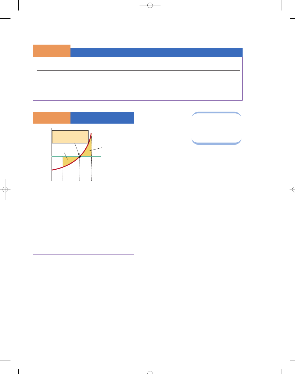
HOW DO FIRMS MAXIMIZE PROFITS?
Now that we have discussed the firm’s cost curves (in
Chapter 12) and its revenues, we are ready to see how
a firm maximizes its profits. A firm’s profits equal its
total revenues minus its total costs. However, at what
output level must a firm produce and sell to maximize
profits? In all types of market environments, the firm
will maximize its profits at the output that maximizes
the difference between total revenue and total cost,
which is at the same output level at which marginal
revenue equals marginal cost.
EQUATING MARGINAL REVENUE
AND MARGINAL COST
The importance of equating marginal revenue and
marginal cost is seen in Exhibit 2. As output expands
beyond zero up to q*, the marginal revenue derived
S E C T I O N
13.3
P r o fi t M a x i m i z a t i o n
■
What is total revenue?
■
What is average revenue?
■
What is marginal revenue?
■
Why does the firm maximize profits where
marginal revenue equals marginal costs?
marginal revenue
(MR)
the increase in total revenue result-
ing from a one-unit increase in sales
total revenue (TR)
the product price times the quan-
tity sold
average revenue (AR)
total revenue divided by the
number of units sold
95469_13_Ch13_p331-364.qxd 29/12/06 12:41 PM Page 337
338
M O D U L E 3
Households, Firms, and Market Structure
from each unit of the expanded output exceeds the
marginal cost of that unit of output; so the expan-
sion of output creates additional profits. This addi-
tion to profit is shown as the leftmost shaded section
in Exhibit 2. As long as marginal revenue exceeds
marginal cost, profits continue to grow. For exam-
ple, if the firm decides to produce q
1
, the firm
sacrifices potential profits, because the marginal rev-
enue from producing more output is greater than the
marginal cost. Only at q*, where MR
MC, is the
output level just right—not too large, not too small.
Further expansion of output beyond q* will lead to
losses on the additional output (i.e., decrease the
firm’s overall profits), because MC
MR. For exam-
ple, if the firm produces q
2
, the firm incurs losses on
the output produced
beyond q*; the firm
should reduce its
output. Only at output
q*, where MR
MC,
can we find the
profit-
maximizing level of
output.
Be careful not to make the mistake of focusing on
profit per unit rather than total profit. That is, you
might think that at q
1
, if MR is much greater than MC,
the firm should not produce more because the profit
per unit is high at this point. However, that would be
a mistake because a firm can add to its total profits as
long as MR > MC—that is, all the way to q*.
The Marginal Approach
We can use the data from the table in Exhibit 3 to find
Farmer Jones’s profit-maximizing position. Columns 5
and 6 show the marginal revenue and marginal cost,
respectively. We see that output levels of 1 and 2 bushels
produce outputs that have marginal revenues that
exceed marginal cost—Farmer Jones wants to produce
those units and more. That is, as long as marginal rev-
enue exceeds marginal cost, producing and selling those
units add more to revenues than to costs; in other
words, they add to profits. However, once he expands
production beyond four units of output, Farmer Jones’s
costs are less than his marginal revenues, and his profits
begin to fall. Clearly, Farmer Jones should not produce
beyond 4 bushels of wheat.
Let’s take another look at profit maximization,
using the table in Exhibit 3. Comparing columns 2 and
3—the calculations of total revenues and total costs,
respectively—we see that Farmer Jones maximizes his
profits at output levels of 3 or 4 bushels, where he will
make profits of $4. In column 4—profit—you can see
that there is no higher level of profit at any of the other
output levels. Producing 5 bushels would reduce prof-
its by $1, because marginal revenue, $5, is less than the
marginal cost, $6. Consequently, Farmer Jones would
not produce this bushel of output. If MR
> MC,
Revenues for a Perfectly Competitive Firm
S E C T I O N
1 3 . 3
E
X H I B I T
1
Quantity
Price
Total Revenue
Average Revenue
Marginal Revenue
(q)
(P)
(TR
P q)
(AR
TR/q)
(MR
TR/q)
1
$5
$ 5
$5
$5
2
5
10
5
5
3
5
15
5
5
4
5
20
5
5
5
5
25
5
Finding the Profit-Maximizing
Level of Output
S E C T I O N
1 3 . 3
E
X H I B I T
2
Price
Lost profit
q
2
q
*
Lost profit
q
1
q
*
MC
q
1
q
*
q
2
P
MR
Quantity of Wheat
(bushels per year)
0
$5
A firm maximizes profits
by producing the quantity
where
MR
MC at q*.
At any output below q*—at q
1
, for example—the mar-
ginal revenue (MR) from expanding output exceeds
the added costs (MC) of that output, so additional
profits can be made by expanding output. Beyond
q*—at q
2
, for example—marginal costs exceed mar-
ginal revenue, so output expansion is unprofitable and
output should be reduced. The profit-maximizing level
of output is at q*, where the profit-maximizing output
rule is followed—the firm should produce the level of
output where MR
MC.
profit-maximizing
level of output
a firm should always produce at the
output where MR
MC
95469_13_Ch13_p331-364.qxd 29/12/06 12:41 PM Page 338

C H A P T E R 1 3
Firms in Perfectly Competitive Markets
339
Farmer Jones should increase production; if MR
< MC,
Farmer Jones should decrease production. Marginal
thinkers make the largest profits.
In the next section we will use the profit-
maximizing output rule to see what happens when
changes in the market cause the price to fall below aver-
age total cost and even below average variable costs. We
will introduce the three-step method to determine
whether the firm is making an economic profit, mini-
mizing its losses, or should be temporarily shut down.
Cost and Revenue Calculations for a Perfectly Competitive Firm
S E C T I O N
1 3 . 3
E
X H I B I T
3
Profit
Marginal Revenue
Marginal Cost
Change in Profit
Quantity Total
Revenue Total
Cost (TR
TC )
(
TR/q)
(
TC/q)
(MR
MC)
(1)
(2)
(3)
(4)
(5)
(6)
(7)
0
$0
$2
$
−2
1
5
4
1
$5
$2
$3
2
10
7
3
5
3
2
3
15
11
4
5
4
1
4
20
16
4
5
5
0
5
25
22
3
5
6
1
S E C T I O N
*
C H E C K
1.
Total revenue is price times the quantity sold (TR
P q).
2.
Average revenue is total revenue divided by the quantity sold (AR
TR/q P).
3.
Marginal revenue is the change in total revenue from the sale of an additional unit of output (MR
TR/q). In a
competitive industry, the price of the good equals both the average revenue and the marginal revenue.
4.
As long as the marginal revenue exceeds marginal costs, the seller should expand production, because producing
and selling those units adds more to revenues than to costs; that is, it increases profits. However, if the marginal
revenue is less than the marginal cost, the seller should decrease production.
5.
The profit-maximizing output rule says a firm should always produce where MR
MC.
1.
How is total revenue calculated?
2.
How is average revenue derived from total revenue?
3.
How is marginal revenue derived from total revenue?
4.
Why is marginal revenue equal to price for a perfectly competitive firm?
S E C T I O N
13.4
S h o r t - R u n P r o fi t s a n d L o s s e s
■
How do we determine whether a firm is
generating an economic profit?
■
How do we determine whether a firm is
experiencing an economic loss?
■
How do we determine whether a firm is
making zero economic profits?
■
Why doesn’t a firm produce when price is
below average variable cost?
In the previous section, we discussed how to de-
termine the profit-maximizing output level for a
perfectly competitive firm. How do we know whether
a firm is actually making economic profits or losses?
95469_13_Ch13_p331-364.qxd 29/12/06 12:41 PM Page 339

340
M O D U L E 3
Households, Firms, and Market Structure
THE THREE-STEP METHOD
What Is the Three-Step Method?
Determining whether a firm is generating economic
profits, economic losses, or zero economic profits at the
profit-maximizing level of output, q*, can be done in
three easy steps. First, we will walk through these steps,
and then we will apply the method to three situations
for a hypothetical firm in the short run in Exhibit 1.
1. Find where marginal revenue equals marginal
cost and proceed straight down to the horizontal
quantity axis to find q*, the profit-maximizing
output level.
2. At q*, go straight up to the demand curve and
then to the left to find the market price, P*.
Once you have identified P* and q*, you can
find total revenue at the profit-maximizing
output level, because TR
P q.
3. The last step is to find the total cost. Again, go
straight up from q* to the average total cost
(ATC) curve and then left to the vertical axis to
compute the average total cost per unit. If we
multiply average total cost by the output level,
we can find the total cost (TC
ATC q).
If total revenue is greater than total cost at q*, the
firm is generating economic profits. If total revenue is
less than total cost at q*, the firm is generating eco-
nomic losses. If total revenue is equal to total cost at
q*, there are zero economic profits (or a normal rate
of return).
Alternatively, to find total economic profits, we
can take the product price at P* and subtract the
average total cost at q*. This will give us per unit
profit. If we multiply this by output, we will arrive at
total economic profit. Or (P*
ATC) q* total
economic profit.
Remember, the cost curves include implicit and
explicit costs—that is, we are covering the opportu-
nity costs of our resources. Therefore, even with zero
economic profits, no tears should be shed, because
the firm is covering both its implicit and explicit
costs. Because firms are also covering their implicit
costs, or what they could be producing with these
resources in another endeavor, economists sometimes
call this zero economic profit a normal rate of return.
That is, the owners are doing as well as they could
elsewhere, in that they are getting the normal rate of
return on the resources they invested in the firm.
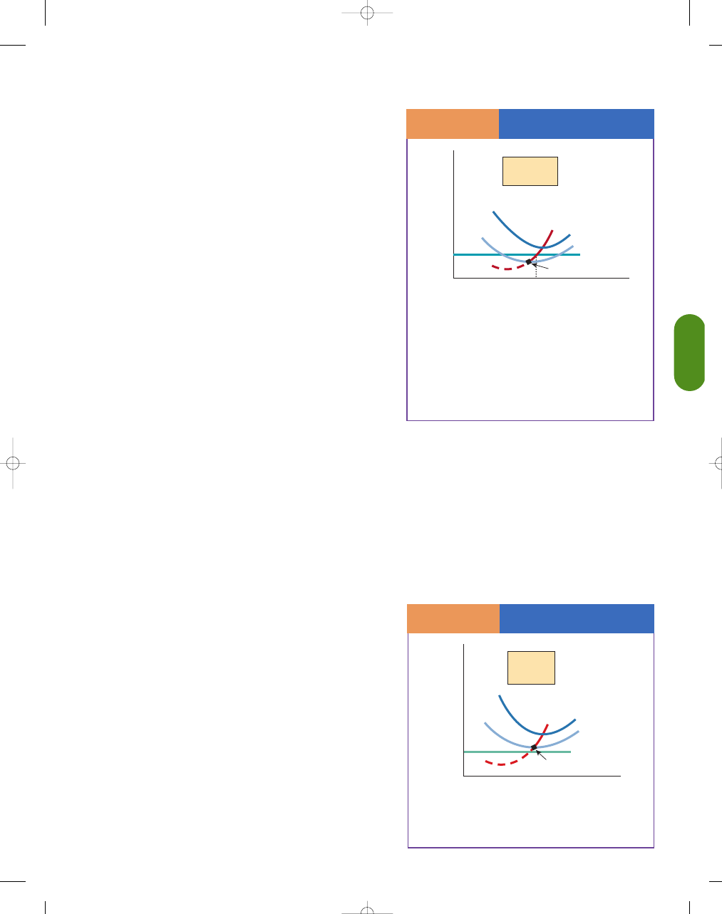
The Three-Step Method in Action
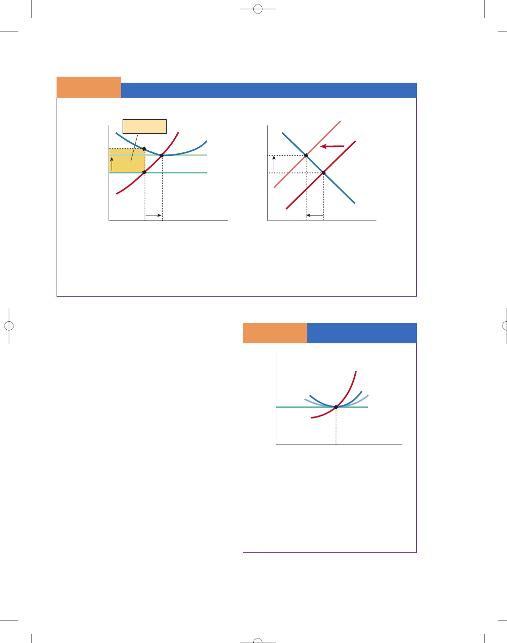
Exhibit 1 shows three different short-run equilibrium
positions; in each case, the firm is producing at a level
where marginal revenue equals marginal cost. Each of
these alternatives shows that the firm is maximizing
profits or minimizing losses in the short run.
Assume that three alternative prices—$6, $5, and
$4—are available for a firm with given costs. In
Exhibit 1(a), the firm receives $6 per unit at an equi-
librium level of output (MR
MC) of 120 units. Total
revenue (P
q*) is $6 120, or $720. The average
total cost at 120 units of output is $5, and the total
cost (ATC
q*) is $600. Following the three-step
method, we can calculate that this firm is earning a
total economic profit of $120. Or we can calculate
total economic profit by using the following equation:
(P*
ATC) q* ($6 $5) 120 $120.
In Exhibit 1(b), the market price has fallen to
$4 per unit. At the equilibrium level of output, the firm
Short-Run Profits, Losses, and Zero Economic Profits
S E C T I O N
1 3 . 4
E
X H I B I T
1
(Profit-Maximizing Output)
0
q
*
100
P
MR
P*
ATC
$4.90
MC
ATC
(Loss-Minimizing Output)
0
q
*
80
Total
Loss
P
MR
ATC
$5
P*
4
MC
ATC
(Profit-Maximizing Output)
0
q
*
120
Total
Profit
P
MR
Price
Price
Price
P*
$6
ATC
5
MC
ATC
P
ATC at q*
Zero Economic
Profit
P
ATC at q*
Economic Profit
P
ATC at q*
Economic Loss
Quantity
Quantity
Quantity
In (a), the firm is earning short-run economic profits of $120. In (b), the firm is suffering losses of $80. In (c), the firm
is making zero economic profits, with the price just equal to the average total cost in the short run.
a. Economic Profit
c. Zero Economic Profits
b. Economic Loss
95469_13_Ch13_p331-364.qxd 29/12/06 12:41 PM Page 340
C H A P T E R 1 3
Firms in Perfectly Competitive Markets
341
is now producing 80 units of output at an average
total cost of $5 per unit. The total revenue is now
$320 ($4
80), and the total cost is $400 ($5 80).
We can see that the firm is now incurring a total eco-
nomic loss of $80. Or we can calculate total economic
profit by using the following equation: (P*
ATC)
q*
($4 $5) 80 $80.
In Exhibit 1(c), the firm is earning zero economic
profits, or a normal rate of return. The market price is
$4.90, and the average total cost is $4.90 per unit for
100 units of output. In this case, economic profits are
zero, because total revenue, $490, minus total cost,
$490, is equal to zero. This firm is just covering all its
costs, both implicit and explicit. Or we can calculate
total economic profit by using the following equation:
(P*
ATC) q* $4.90 $4.90 100 $0.
EVALUATING ECONOMIC LOSSES
IN THE SHORT RUN
A firm generating an economic loss faces a tough
choice: Should it continue to produce or should it
shut down its operation? To make this decision, we
need to add another variable to our discussion of eco-
nomic profits and losses: average variable cost.
Variable costs are costs that vary with output—for
example, wages, raw material, transportation, and
electricity. If a firm cannot generate enough revenues
to cover its variable costs, it will have larger losses if
it operates than if it shuts down (when losses are
equal to fixed costs). That is, the firm will shut down
if its total revenue (p
q) is less then its variable costs
(VC). If we divide p
q by q, we get p, and if we
divide VC by q we get AVC, so if p
AVC, a profit-
maximizing firm will shut down. Thus, a firm will not
produce at all unless the price is greater than its aver-
age variable cost.
Operating at a Loss
At price levels greater than or equal to the average
variable cost, a firm may continue to operate in the
short run even if its average total cost—variable and
fixed costs—is not completely covered. That is, the
firm may continue to operate even though it is expe-
riencing an economic loss. Why? Because fixed costs
continue whether the firm produces or not; it is better
to earn enough to cover a portion of fixed costs than
to earn nothing at all.
In Exhibit 2, price is less than average total cost
but more than average variable cost. In this case, the
firm produces in the short run, but at a loss. To shut
down would make this firm worse off, because it can
cover at least some of its fixed costs with the excess of
revenue over its variable costs.
The Decision to Shut Down
Exhibit 3 illustrates a situation in which the price a
firm is able to obtain for its product is below its
average variable cost at all ranges of output. In this
case, the firm is unable to cover even its variable
costs in the short run. Because the firm is losing even
more than the fixed costs it would lose if it shut
down, it is more logical for the firm to cease opera-
tions. Hence, if P
AVC, the firm can cut its losses
by shutting down.
Short-Run Losses: Price
Above AVC But Below ATC
S E C T I O N
1 3 . 4
E
X H I B I T
2
Quantity
(firm)
0
Price
q
P
MC
ATC
AVC
Shutdown Point
P
AVC
Firm should not
shut down
P
MR
In this case, the firm operates in the short run but
incurs a loss because P
ATC. Nevertheless, P AVC,
and revenues cover variable costs and partially defray
fixed costs. This firm will leave the industry in the
long run unless prices are expected to rise in the near
future; but in the short run, it continues to operate at
a loss as long as P
AVC, the shutdown point.
Short-Run Losses:
Price Below AVC
S E C T I O N
1 3 . 4
E
X H I B I T
3
Quantity
0
Price
P
MC
ATC
AVC
P
⫽ MR
Shutdown Point
P
⬍
AVC
Firm should
shut down
Because its average variable cost exceeds price at all levels
of output, this firm would cut its losses by discontinuing
production.
95469_13_Ch13_p331-364.qxd 29/12/06 12:41 PM Page 341

342
M O D U L E 3
Households, Firms, and Market Structure
The Short-Run Supply Curve
As we have just seen, at all prices above the minimum
AVC, a firm produces in the short run even if average
total cost (ATC) is not completely covered; and at all
prices below the minimum AVC, the firm shuts down.
The firm produces above the minimum AVC even if it
is incurring economic losses because it can still earn
enough in total revenues to cover all its average vari-
able cost and a portion of its fixed costs, which is
better than not producing and earning nothing at all.
In graphical terms, the
short-run supply curve
of an individual competitive seller is identical to the
portion of the MC curve that lies above the minimum
of the AVC curve. As a
cost relation, this curve
shows the marginal
cost of producing any
given
output;
as
a
supply curve, it shows
the equilibrium output
that
the
firm
will
supply at various prices in the short run. The thick
line in Exhibit 4 is the firm’s supply curve—the por-
tion of MC above its intersection with AVC. The
declining portion of the MC curve has no
significance for supply, because if the price falls
below the average variable cost, the firm is better off
shutting down—producing no output. The shutdown
point is at the minimum point on the average variable
cost curve where the output level is q
SHUT DOWN
.
Beyond the point of lowest AVC, the marginal costs
of successively larger amounts of output are pro-
gressively greater, so the firm will supply larger and
larger amounts only at higher prices. The absolute
maximum that the firm can supply, regardless of
price, is the maximum quantity that it can produce
with the existing plant.
DERIVING THE SHORT-RUN MARKET SUPPLY CURVE
The
short-run market supply curve
is the sum-
mation of all the individual firms’ supply curves
(that is, the portion of
the firms’ MC above
AVC) in the market.
Because the short run
is too brief for new
firms to enter the
market, the market
supply curve is the
summation of existing
firms. For example, in Exhibit 5, at P
1
, each of the
1,000 identical firms in the industry produces 500
bushels of wheat per day at point a, in Exhibit 5(a);
and the quantity supplied in the market is 500,000
bushels of wheat, point A, in Exhibit 5(b). We can
again sum horizontally at P
2
; the quantity supplied
for each of the 1,000 identical firms is 800 bushels
of wheat per day at point b in Exhibit 5(a), so the
quantity supplied for the industry is 800,000 bushels
Because the demand for summer camps will be lower during
the off-season, it is likely that revenues may be too low for
the camp to cover its variable costs and the owner will
choose to shut down. Remember, the owner will still have to
pay the fixed costs: property tax, insurance, the costs associ-
ated with the building and land. However, if the camp is not
in operation during the off-season, the owner will at least
not have to pay the variable costs: salaries for the camp staff,
food, and electricity.
The Firm’s Short-Run
Supply Curve
S E C T I O N
1 3 . 4
E
X H I B I T
4
Quantity
0
Price
Short-Run Supply
MC
AVC
P
MIN
q
SHUT DOWN
ATC
Firms shut down
if
P < AVC
If price is less than average variable cost, the firm’s
losses would be smaller if it shut down and stopped
producing. That is, if P
AVC, the firm is better off
producing zero output. Hence, the firm’s short-run
supply curve is the marginal cost curve above average
variable cost.
short-run market
supply curve
the horizontal summation of the
individual firms’ supply curves in
the market
short-run supply
curve
the portion of the MC curve above
the AVC curve
95469_13_Ch13_p331-364.qxd 29/12/06 12:41 PM Page 342

C H A P T E R 1 3
Firms in Perfectly Competitive Markets
343
Deriving the Short-Run Market Supply Curve
S E C T I O N
1 3 . 4
E
X H I B I T
5
Quantity of Wheat
(bushels per day)
0
500
800
b
a
B
A
P
2
P
1
Individual
Firm
Supply (
MC )
Quantity of Wheat
(bushels per day)
0
500,000
800,000
P
2
P
1
P
AVC
P
AVC
Market
Supply
Price per Bushel
Price per Bushel
A
B
The short-run supply curve is the horizontal summation of the individual firms’ supply curves (each firm’s marginal
cost curve above AVC), shown in (a). In a market of 1,000 identical wheat farmers, the market supply curve is 1,000
times the quantity supplied by each firm, shown in (b).
a. Individual Firm Supply Curve for Wheat
b. Market Supply Curve for Wheat
using what you’ve learned
Evaluating Short-Run Economic Losses
Lei-ann is one of many florists in a medium-size urban area. That is,
we assume that she works in a market similar to a perfectly com-
petitive market and operates, of course, in the short run. Lei-ann’s cost and
revenue information is shown in Exhibit 6. Based on this information, what
should Lei-ann do in the short run, and why?
Fixed costs are unavoidable unless the firm goes out of business. Lei-ann
really has two decisions in the short run—either to operate or to shut
down temporarily. In Exhibit 6, we see that Lei-ann makes $2,000 a day in total
revenue, but her daily costs (fixed and variable) are $2,500. She has to pay her
workers, pay for fresh flowers, and pay for the fuel used by her drivers in picking
up and delivering flowers. She must also pay the electricity bill to heat her shop
and keep her refrigerators going to protect her flowers. That is, every day, poor
Lei-ann is losing $500; but she still might want to operate the shop despite the
loss. Why? Lei-ann’s average variable cost (comprising flowers, transportation,
fuel, daily wage earners, and so on) amounts to $1,500 a day; her fixed costs
(insurance, property taxes, rent for the building, and refrigerator payments) are
$1,000 a day. Now, if Lei-ann does not operate, she will save on her variable cost—
$1,500 a day—but she will be out the $2,000 a day she makes in revenue from sell-
ing her flowers. Thus, every day she operates, she is better off than if she had not
operated at all. That is, if the firm can cover the average variable cost, it is better
off operating than not operating. But suppose Lei-ann’s VC were $2,100 a day.
Then Lei-ann should not operate, because every day she does, she is $100 worse
off than if she shut down altogether. In short, a firm will shut down if TR < VC
or (P
q)<VC. If we divide both sides by q,the firm will shut down if P <AVC
or (P
q)/q < VC/q.
Why does Lei-ann even bother operating if she is making a loss? Perhaps
the economy is in a recession and the demand for flowers is temporarily
down, but Lei-ann thinks things will pick up again in the next few months.
If Lei-ann is right and demand picks up, her prices and marginal revenue will
rise, and she may have a chance to make short-run economic profits.
Q
A
If Lei-ann cannot cover her fixed costs, will she continue to operate?
Lei-ann’s Daily Revenue
and Cost Schedule
S E C T I O N
1 3 . 4
E
X H I B I T
6
Total Revenue
$2,000
Total Costs
2,500
Variable Costs
1,500
Fixed Costs
1,000
95469_13_Ch13_p331-364.qxd 29/12/06 12:41 PM Page 343
344
M O D U L E 3
Households, Firms, and Market Structure
using what you’ve learned
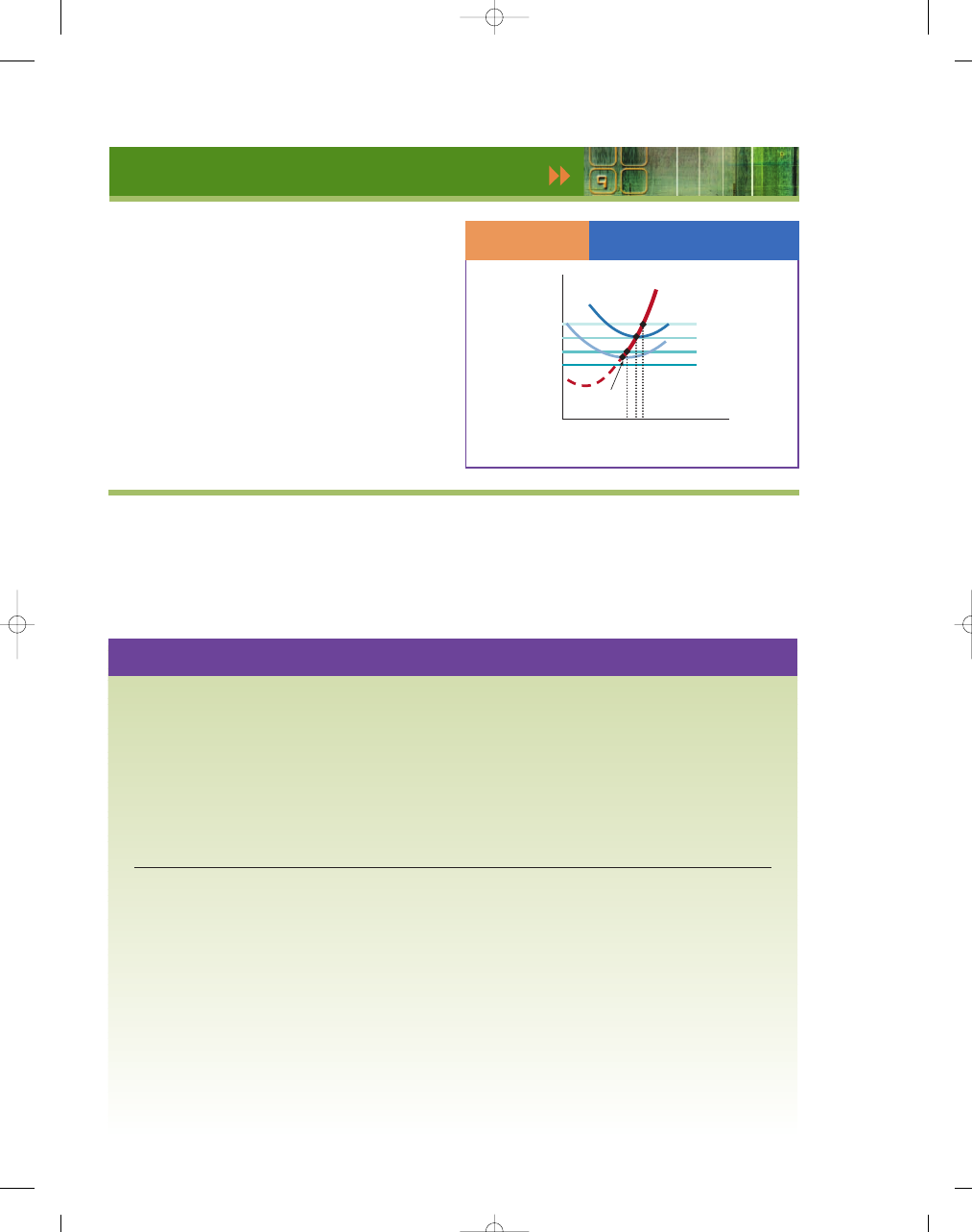
Reviewing the Short-Run Output Decision
Exhibit 7 shows the firm’s short-run output at these various market prices: P
1
,
P
2
, P
3
, and P
4
.
At the market price of P
1
, the firm would not cover its average variable
cost—the firm would produce zero output, because the firm’s losses would be
smaller if it shut down and stopped producing. At the market price of P
2
, the
firm would produce at the loss-minimizing output of q
2
units. It would oper-
ate rather than shut down, because it could cover all its average variable cost
and some of its fixed costs. At the market price of P
3
, the firm would produce
q
3
units of output and make zero economic profit (a normal rate of return). At
the market price of P
4
, the firm would produce q
4
units of output and be
making short-run economic profits.
The Short-Run
Output Decision
S E C T I O N
1 3 . 4
E
X H I B I T
7
0
Price
Shutdown
point
P
1
q
2
q
3
q
4
P
2
P
3
P
4
d
4
,
mr
4
d
3
,
mr
3
d
2
,
mr
2
d
1
,
mr
1
MC
ATC
AVC
Quantity
S E C T I O N
*
C H E C K
1.
The profit-maximizing output level is found by equating MR to MC at q*. If at that output the firm’s price is greater
than its average total costs, it is making an economic profit.
2.
If at the profit-maximizing output level, q*, the price is less than the average total cost, the firm is incurring an eco-
nomic loss.
3.
If at the profit-maximizing output level, q*, the price is equal to average total cost, the firm is making
zero economic profits; that is, the firm is covering both its implicit and explicit costs (making a normal rate
of return).
4.
If the price falls below average variable cost, the firm is better off shutting down than operating in the short run,
because it would incur greater losses from operating than from shutting down.
1.
How is the profit-maximizing output quantity determined?
2.
How do we determine total revenue and total cost for the profit-maximizing output quantity?
3.
If a profit-maximizing perfectly competitive firm is earning a profit because total revenue exceeds total cost,
why must the market price exceed average total cost?
4.
If a profit-maximizing perfectly competitive firm is earning a loss because total revenue is less than total cost, why
must the market price be less than average total cost?
5.
If a profit-maximizing perfectly competitive firm is earning zero economic profits because total revenue equals
total cost, why must the market price be equal to the average total cost for that level of output?
6.
Why would a profit-maximizing perfectly competitive firm shut down rather than operate if price was less than its
average variable cost?
7.
Why would a profit-maximizing perfectly competitive firm continue to operate for a period of time if price was
greater than average variable cost but less than average total cost?
of wheat per day, point B in Exhibit 5(b).
Continuing this process gives us the market supply
curve for the wheat market. In a market of 1,000
identical wheat farmers, the market supply curve is
1,000 times the quantity supplied by each firm, as
long as the price is above AVC.
95469_13_Ch13_p331-364.qxd 29/12/06 12:41 PM Page 344
C H A P T E R 1 3
Firms in Perfectly Competitive Markets
345
ECONOMIC PROFITS AND LOSSES DISAPPEAR
IN THE LONG RUN
If farmers are able to make economic profits produc-
ing wheat, what will their response be in the long run?
Farmers will increase the resources that they devote to
the lucrative business of producing wheat. Suppose
Farmer Jones is making an economic profit (he is
earning an above-normal rate of return) producing
wheat. To make even more profits, he may take land
out of producing other crops and plant more wheat.
Other farmers or people who are holding land for
speculative purposes may also decide to plant wheat
on their land.
As word gets out that wheat production is prov-
ing profitable, it will cause a supply response—the
market supply curve will shift to the right as more
firms enter the industry and existing firms expand as
shown in Exhibit 1(b). With this shift, the quantity of
wheat supplied at any given price is greater than
before. It may take a year or even longer, of course,
for the complete supply response to take place, simply
because it takes some time for information on profit
opportunities to spread and still more time to plant,
grow, and harvest the wheat. Note that the effect of
increasing supply, other things being equal, is a reduc-
tion in the equilibrium price of wheat.
Suppose that, as a result of the supply response,
the price of wheat falls from P
1
to P
2
. The impact of
the change in the market price of wheat, over which
Farmer Jones has absolutely no control, is simple. If
his costs don’t change, he moves from making a profit
(P
1
ATC) to zero economic profits (P
2
ATC), as
shown in Exhibit 1(a). In long-run equilibrium, per-
fectly competitive firms make zero economic profits.
Remember, a zero economic profit means that the
firm actually earns a normal return on the use of its
capital. Zero economic profit is an equilibrium or
stable situation because any positive economic
(above-normal) profit signals resources into the
industry, beating down prices and therefore revenues
to the firm.
S E C T I O N
13.5
L o n g - R u n E q u i l i b r i u m
■
When an industry is earning profits, will it
encourage the entry of new firms?
■
Why do perfectly competitive firms make
zero economic profits in the long run?
Profits Disappear with Entry
S E C T I O N
1 3 . 5
E
X H I B I T
1
Quantity
0
Price
Q
1
Q
2
P
1
P
2
S
1
D
S
2
Quantity
0
q
2
q
1
d
1
,
mr
1
d
2
, mr
2
P
1
P
2
Price
MC
ATC
ATC
Economic Profits
P
1
>
ATC at
q
1
As the industry-determined price of wheat falls in (b), Farmer Jones’s marginal revenue curve shifts downward from
mr
1
to mr
2
in (a). A new profit-maximizing (MC
MR) point is reached at q
2
. When the price is P
1
, Farmer Jones is
making a profit, because P
1
ATC. When the market supply increases, causing the market price to fall to P
2
, Farmer
Jones’s profits disappear, because P
2
ATC.
a. Individual Firm
b. Market
95469_13_Ch13_p331-364.qxd 29/12/06 12:41 PM Page 345
346
M O D U L E 3
Households, Firms, and Market Structure
Any economic losses signal resources to leave the
industry, causing supply reductions that lead to
increased prices and higher firm revenues for the
remaining firms. For example, in Exhibit 2 we see a
firm that continues to operate despite its losses—ATC
is greater than P
1
at q
1
. With losses, however, some
firms will exit the industry, causing the market supply
curve to shift from S
1
to S
2
and driving up the market
price to P
2
. This price increase reduces the losses for
the firms remaining in the industry, until the losses are
completely eliminated at P
2
. The remaining firms will
maximize profits by producing at q
2
units of output,
where profits and losses are zero. Only at zero eco-
nomic profits is there no tendency for firms to either
enter or leave the industry.
THE LONG-RUN EQUILIBRIUM
FOR THE COMPETITIVE FIRM
The long-run competitive equilibrium for a perfectly
competitive firm is illustrated graphically in Exhibit 3.
At the equilibrium point, e (where MC
MR),
short-run and long-run average total costs are also
equal. The average total cost curves touch the mar-
ginal cost and marginal revenue (demand) curves at
the equilibrium output point. Because the marginal
revenue curve is also the average revenue curve,
average revenue and average total cost are equal at
the equilibrium point. The long-run equilibrium in
perfect competition depicted in Exhibit 3 has an
interesting feature. Note that the equilibrium output
Losses Disappear with Exit
S E C T I O N
1 3 . 5
E
X H I B I T
2
Quantity
a. Individual Firm
b. Market
0
q
1
q
2
d
2
, mr
2
d
1
, mr
1
MC
ATC
ATC
P
2
P
1
Economic Losses
ATC
P
1
at
q
1
Quantity
0
Q
2
Q
1
S
1
S
2
D
P
2
P
1
When firms in the industry suffer losses, some firms will exit in the long run, shifting the market supply curve
to the left from S
1
to S
2
. This shift causes market price to rise from P
1
to P
2
and market output to fall from
Q
1
to Q
2
. When the price is P
1
, the firm is incurring a loss, because ATC is greater than P
1
at q
1
. When the
market supply increases from S
1
to S
2
, it causes the market price to rise and the firm’s losses disappear, because
P
2
ATC.
The Long-Run
Competitive Equilibrium
S E C T I O N
1 3 . 5
E
X H I B I T
3
Quantity of Wheat
(bushels per year)
0
Price
q*
$10
MC
LRATC
P
MR
SRATC
e
In the long run in perfect competition, a stable situa-
tion or equilibrium is achieved when economic profits
are zero. In this case, at the profit-maximizing point
where MC
MR, short-run and long-run average total
costs are equal. Industrywide supply shifts would change
prices and average revenue, wiping out any losses or
profits that develop in the short run and leading to the
situation depicted in the exhibit.
95469_13_Ch13_p331-364.qxd 29/12/06 12:41 PM Page 346

C H A P T E R 1 3
Firms in Perfectly Competitive Markets
347
occurs at the lowest point on the average total cost
curve. As you may recall, this occurs because the
marginal cost curve must intersect the average total
cost curve at the latter curve’s lowest point. Hence,
the equilibrium condition in the long run in perfect
competition is for each firm to produce at the output
that minimizes average total cost—that is, the firm is
operating at its minimum efficient scale. At this
long-run equilibrium, all firms in the industry earn
zero economic profit; consequently, new firms have
no incentive to enter the market, and existing firms
have no incentive to exit the market.
i n t h e n e w s
The Gaming Market
Nevada bettors wagered a combined $71.7 million, up slightly from last year’s
handle of $71.5 million. [There are] a number of potential problems facing the
state’s gaming industry, most notably increased competition from Indian
gaming and Internet-based sports wagering services. . . .
Bettor’s increased use of offshore sports books no doubt reduced the
handle at Nevada’s sports books, said Frank Streshley, senior researcher for the
Gaming Control Board.
“Obviously, six or seven years ago, you didn’t have that competition to
our books,” Streshley said.
SOURCE: Chris Jones, “Super Bowl Betting Exposes Potential Woes for Nevada
Casino Industry,” Las Vegas Review Journal, 30 January 2003.
CONSIDER THIS:
In reality, few markets fit all the criteria of a perfectly competitive
market—large numbers of buyers and sellers, homogeneous goods,
easy entry, and perfect information. Agricultural markets probably
come the closest, but still many agricultural markets have some form
of market imperfection. However, just because an industry may not
fully satisfy all the conditions of perfect competition, the model is
still useful.
Consider the gaming market, for example. It certainly cannot be
considered a precise example of a perfectly competitive market.
However, the model can still be useful, especially when considering
the many buyers and sellers and the entry and exit aspects of the
market. To a lesser extent, they are all selling pretty much the same
product. Of course, gambling comes with more bells and whistles in
Las Vegas.
The gaming industry was almost exclusively Nevada’s in the 1960s
and 1970s. Now, many more sellers include Atlantic City casinos, legal
lottos, casinos on Native American reservations, river boat and cruise
ship gambling, and Internet betting. Add to that the thousands of
bookies all over the country, some illegally placing the bets them-
selves and others using messengers in legal sites such as Las Vegas and
Atlantic City. The point is this: The industry was once dominated by a
few but has become much more competitive, with the profits now
being shared with many new competitors that have provided viable
substitutes.
S E C T I O N * C H E C K
1.
Economic profits encourage the entry of new firms, which shift the market supply curve to the right.
2.
Any positive economic profits signal resources into the industry, driving down prices and revenues to the firm.
3.
Any economic losses signal resources to leave the industry, leading to supply reduction, higher prices, and
increased revenues.
4.
Only at zero economic profits is there no tendency for firms to either enter or exit the industry.
1.
Why do firms enter profitable industries?
2.
Why does entry eliminate positive economic profits in a perfectly competitive industry?
©
ASSOCIA
TED PRESS
95469_13_Ch13_p331-364.qxd 29/12/06 12:42 PM Page 347

348
M O D U L E 3
Households, Firms, and Market Structure
The preceding sections considered the costs for an
individual, perfectly competitive firm as it varies
output, on the assumption that the prices it pays for
inputs (costs) are given. However, when the output
of an entire industry changes, the likelihood is
greater that changes in costs will occur. How will the
changes in the number of firms in an industry affect
the input costs of individual firms? In this section,
we develop the long-run supply (LRS) curve. As we
will see, the shape of the long-run supply curve
depends on the extent to which input costs change
with the entry or exit of firms in the industry. We
will look at three possible types of industries when
considering long-run supply: constant-cost indus-
tries, increasing-cost industries, and decreasing-cost
industries.
A CONSTANT-COST INDUSTRY
In a
constant-cost industry,
the prices of inputs do
not change as output is expanded. The industry may
not use inputs in
sufficient quantities to
affect input prices. For
example, say the firms
in the industry use a lot
of unskilled labor but
the industry is small.
Therefore, as output
expands, the increase in
demand for unskilled labor will not cause the market
wage for unskilled labor to rise. Similarly, suppose a
paper clip maker decides to double its output. It is
highly unlikely that its demand for steel will have an
impact on steel prices, because its demand for the
input is so small.
Once long-run adjustments are complete, by
necessity each firm operates at the point of lowest
long-run average total cost, because supply shifts with
entry and exit, eliminating profits. Therefore, each
firm supplies the market with the quantity of output
that it can produce at the lowest possible long-run
average total cost.
In Exhibit 1, we can see the impact of an unex-
pected increase in market demand. Suppose that
recent reports show that blueberries can lower cho-
lesterol, lower blood pressure, and significantly
reduce the risk of all cancers. The increase in market
demand for blueberries leads to a price increase from
P
1
to P
2
as the firm increases output from q
1
to q
2
,
and blueberry industry output increases from Q
1
to
Q
2
, as seen in Exhibit 1(b). The increase in market
demand generates a higher price and positive profits
for existing firms in the short run. The existence of
economic profits will attract new firms into the indus-
try, causing the short-run supply curve to shift from S
1
to S
2
and lowering price until excess profits are zero.
This shift results in a new equilibrium, point C in
Exhibit 1(c). Because the industry is one with
constant costs, industry expansion does not alter
firms’ cost curves, and the industry long-run supply
curve is horizontal. That is, the long-run equilibrium
price is at the same level that prevailed before demand
increased; the only long-run effect of the increase in
demand is an increase in industry output, as more
firms enter that are just like existing firms [shown in
Exhibit 1(c)]. However, the long-run supply curve
does not have to be horizontal.
3.
Why do firms exit unprofitable industries?
4.
Why does exit eliminate economic losses in a perfectly competitive industry?
5.
Why is a situation of zero economic profits a stable long-run equilibrium situation for a perfectly competitive
industry?
S E C T I O N
13.6
L o n g - R u n S u p p l y
■
What are constant-cost industries?
■
What are increasing-cost industries?
■
What are decreasing-cost industries?
■
What is productive efficiency?
■
What is allocative efficiency?
constant-cost
industry
an industry where input prices (and
cost curves) do not change as indus-
try output changes
95469_13_Ch13_p331-364.qxd 29/12/06 12:42 PM Page 348

C H A P T E R 1 3
Firms in Perfectly Competitive Markets
349
Demand Increase in a Constant-Cost Industry
S E C T I O N
1 3 . 6
E
X H I B I T
1
Quantity of Blueberries
(market)
0
B
C
A
Price of
Blueberries
Q
2
Q
1
Q
3
P
2
P
1
S
1
D
2
D
1
S
2
LRS
Quantity of Blueberries
(firm)
0
b
a, c
Price of
Blueberries
q
1
q
2
d
2
, mr
2
d
1
, mr
1
P
2
P
1
SRMC
ATC
Quantity of Blueberries
(market)
0
B
A
Price of
Blueberries
Q
2
Q
1
P
2
P
1
Supply
D
2
D
1
Quantity of Blueberries
(firm)
0
b
a
a
Price of
Blueberries
q
1
q
2
d
2
,
mr
2
d
1
,
mr
1
P
2
P
1
SRMC
ATC
Total Profits
Quantity of Blueberries
(market)
0
A
Price of
Blueberries
Q
1
P
1
Supply
Demand
Quantity of Blueberries
(firm)
0
Price of
Blueberries
q
1
d
1
,
mr
1
P
1
SRMC
ATC
a. Initial Equilibrium
b. Short-Run Profits
c. Long-Run Entry and No Economic Profits
An unexpected increase in market demand for blueberries leads to an increase in the market price in (b).
The new market price leads to positive profits for existing firms, which attracts new firms into the industry,
shifting market supply from S
1
to S
2
in (c). This increased short-run industry supply curve intersects D
2
at
point C. Each firm (of a new, larger number of firms) is again producing at q
1
and earning zero economic
profits.
95469_13_Ch13_p331-364.qxd 29/12/06 12:42 PM Page 349

i n t h e n e w s
Internet Cuts Costs and Increases Competition
The Internet makes it easier for buyers and sellers to compare prices. It cuts
out the middlemen between firms and customers. It reduces transaction costs
[and] reduces barriers to entry. . . .
To understand this, we could look back to the theories of Ronald
Coase, an economist who argued in 1937 that the main reason why firms
exist (as opposed to individuals acting as buyers and sellers at every stage
of production) is to minimize transaction costs. Since the Internet reduces
such costs, it also reduces the optimal size of firms. Small firms can buy in
services from outside more cheaply. Thus, in overall terms, barriers to entry
will fall.
In these ways, then, the Internet cuts costs, increases competition and
improves the functioning of the price mechanism. It thus moves the economy
closer to the textbook model of perfect competition, which assumes abun-
dant information, zero transaction costs, and no barriers to entry. The Internet
makes this assumption less far-fetched. By improving the flow of information
between buyers and sellers, it makes markets more efficient and so ensures
that resources are allocated to their most productive use. The most important
effect of the “new” economy, indeed, may be to make the “old” economy
more efficient. . . .
It is hard to test this conclusion, but some studies seem to support it.
Prices of goods bought online, such as books and CDs, are, on average, about
10 percent cheaper (after including taxes and delivery) than in conventional
shops, though the non-existent profits of many electronic retailers make this
evidence inconclusive. Competition from the Internet is also forcing tradi-
tional retailers to reduce prices. The Internet offers even clearer savings in
services such as banking. According to Lehman Brothers, a transfer between
bank accounts costs $1.27 if done by a bank teller, 27 cents via cash machine,
and only one cent over the Internet.
SOURCE: “Internet Economics: A Thinker’s Guide,” The Economist, 1 April 2001,
pp. 64–66. © The Economist Newspaper, Ltd. All rights reserved. Reprinted with
permission. Further reproduction prohibited. Http://www.economist.com.
350
M O D U L E 3
Households, Firms, and Market Structure
AN INCREASING-COST INDUSTRY
In an
increasing-cost industry
—a more likely sce-
nario—the cost curves of individual firms rise as the
total output of the
industry increases.
Increases in input prices
(upward shifts in cost
curves) occur as larger
quantities of factors are
employed in the indus-
try. When an industry
utilizes a large portion
of an input whose total supply is not huge, input prices
will rise when the industry uses more of the input.
For example, if a construction boom occurs in a
fully employed economy, would it be more costly to
obtain additional resources such as workers and raw
materials? Yes, as an increasing-cost industry, the
industry can only produce more output if it gets a
higher price, because the firm’s costs of production
rise as output expands. As new firms enter and output
expands, the increase in demand for inputs causes the
price of inputs to rise—the cost curves of all con-
struction firms shift upward as the industry expands.
The industry can produce more output, but only at a
higher price, enough to compensate the firm for the
higher input costs. In an increasing-cost industry, the
long-run supply curve is upward sloping.
Another example is provided by the airlines.
Growth in the airline industry results in more conges-
tion of airports and airspace. This situation is what
economists call external diseconomies—factors that
are beyond the firm’s control that raise the firm’s costs
as industry output expands. That is, as the output of
the airline industry increases, the firm’s cost increases,
ceteris paribus.
A DECREASING-COST INDUSTRY
It is also possible that an expansion in the output of an
industry can lead to a reduction in input costs and shift
the MC and ATC curves downward, and the market
price falls. That is, a firm experiences lower cost as an
industry expands. The new long-run market equilib-
rium has more output at a lower price—that is, the
long-run supply curve for a decreasing-cost industry is
downward sloping (not shown).
As a practical matter, decreasing-cost industries
are rarely encountered, at least over a large range of
output. However, some industries may operate under
decreasing-cost conditions in the short intervals of
output expansion when continued growth makes pos-
sible the supply of materials or services at reduced
cost. A larger industry might benefit from improved
transportation or financial services, for example.
This situation might occur in the computer
industry. The firms in the industry may be able to
acquire computer chips at a lower price as the indus-
try’s demand for computer chips rises. Why?
Perhaps it is because the computer chip industry can
employ cost-saving techniques that become more
increasing-cost
industry
an industry where input prices rise
(and cost curves rise) as industry
output rises
95469_13_Ch13_p331-364.qxd 29/12/06 12:42 PM Page 350
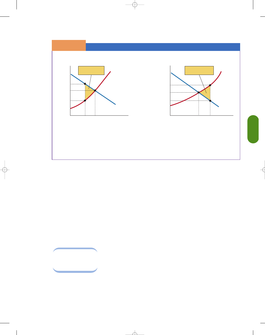
C H A P T E R 1 3
Firms in Perfectly Competitive Markets
351
Allocative Efficiency and Perfect Competition
S E C T I O N
1 3 . 6
E
X H I B I T
2
Quantity
Price
Price
0
MB
MC
P*
S
MC
D
MB
Quantity
0
MC
Q*
Q
2
Q*
MB
P*
S
MC
D
MB
Q
1
Deadweight loss
—too little output
Deadweight loss
—too much output
The demand curve measures the marginal benefits to the consumer and the supply curve measures the marginal
cost to the sellers. At P* and Q*, resources are being allocated efficiently—the marginal benefits of these
resources are equal to the marginal cost of these resources. If Q
1
is produced, then the marginal benefits from
producing additional units are greater than the marginal costs. Society gains from expending output up to the
point where MB
MC at Q*. If output is expanded beyond Q* (MC MB) society gains from a reduction in
output back to Q*.
a. Producing Less Than the Competitive Level of
Output Lowers Welfare
b. Producing More Than the Competitive Level of
Output Lowers Welfare
economical at higher levels of output. That is, the
marginal and average costs of the firm fall as input
prices fall because of expanded output in the indus-
try. In this case, the LRS curve would be negatively
sloped (not shown).
PERFECT COMPETITION AND
ECONOMIC EFFICIENCY
In this chapter, we have seen that a firm in a perfectly
competitive market produces at the minimum of the
ATC curve in the long run and charges a price consis-
tent with that cost. Because competitive firms are pro-
ducing using the least cost method, the minimum
amount of resources is being used to produce a given
level of output. This
leads to lower product
prices for consumers.
In short,
productive
efficiency
requires
that firms produce
goods and services in
the least costly way, where P
Minimum ATC, as
seen in Exhibit 3, on p. 346. However, productive
efficiency alone does not guarantee that markets are
operating efficiently—society must also produce the
goods and services that society wants most. This leads
us to what economists call allocative efficiency.
We say that the output that results from equilib-
rium conditions of market demand and market supply
in perfectly competitive markets achieve an efficient
allocation of resources.
At the intersection of market supply and market
demand, we find the competitive equilibrium price, P*,
and the competitive equilibrium output, Q*. In compet-
itive markets, market supply equals market demand, and
P
MC. When P MC, buyers value the last unit of
output by the same amount that it cost sellers to produce
it. If buyers value the last unit by more than the marginal
cost of production, resources are not being allocated
efficiently, as at Q
1
in Exhibit 2(a). Think of the demand
curve as the marginal benefit curve (D
MB) and the
supply curve as the marginal cost curve (S
MC).
According to the rule of rational choice, we should
pursue an activity as long as the expected marginal
benefits are greater than the expected marginal costs. For
example, in Exhibit 2(a), if Q
1
is produced, then the
marginal benefits from producing additional units are
greater than the marginal costs. The shaded area is
deadweight loss. That is, at Q
1
, resources are not being
allocated efficiently, and output should be expanded.
We can also produce too much output. For exam-
ple, if output is expanded beyond Q* in Exhibit 2(b),
the cost to sellers for producing the good is greater
than the marginal benefit to consumers. The shaded
area is deadweight loss. Society would gain from a
productive efficiency
where a good or service is produced
at the lowest possible cost
95469_13_Ch13_p331-364.qxd 29/12/06 12:42 PM Page 351

352
M O D U L E 3
Households, Firms, and Market Structure
S E C T I O N
*
C H E C K
1.
In constant-cost industries, the cost curves of the firm are not affected by changes in the output of the entire
industry. Such industries must be small demanders of resources in the market.
2.
In an increasing-cost industry, the cost curves of the individual firms rise as total output increases. This case is the
most typical.
3.
A decreasing-cost industry has a downward-sloping long-run supply curve. Firms experience lower cost as industry
expands.
4.
Productive efficiency occurs in perfect competition because the firm produces at the minimum of the ATC curve.
5.
Allocative efficiency occurs when P
MC; production is allocated to reflect consumers' wants.
1.
What must be true about input costs as industry output expands for a constant-cost industry?
2.
What must be true about input costs as industry output expands for an increasing-cost industry?
3.
What would be the long-run equilibrium result of an increase in demand in a constant-cost industry?
4.
What would be the long-run equilibrium result of an increase in demand in an increasing-cost industry?
reduction in output back to Q*. Once the competi-
tive equilibrium is reached, the buyers’ marginal
benefit equals the sellers’ marginal cost. That is, in a
competitive market, producers efficiently use their
scarce resources (labor, machinery, and other inputs)
to produce what con-
sumers want. In this
sense, perfect competi-
tion achieves
alloca-
tive efficiency.
allocative efficiency
where P
MC and production will
be allocated to reflect consumer
preferences
I n t e r a c t i v e S u m m a r y
Fill in the blanks:
1. Economists have identified four different market
structures in which firms operate:
,
, ,
and .
2. Perfect competition is a market structure involving
a(n)
number of buyers and
sellers, a(n)
product, and
market entry and exit.
3. Perfectly competitive firms are
,
who must accept the market price as determined by
the forces of demand and supply.
4. In
, a single seller sets the price
that will maximize the seller’s profits.
5. Monopolistic competition contains an element of
monopoly power because each firm’s product is
from that of other competitors,
but because the market includes
competitors, it also has an element of competition.
6. In oligopoly,
firms, as opposed to
one firm or many, produce similar or identical goods.
7. Because perfectly competitive markets have
buyers and sellers, each firm is
so
in relation to the industry that
its production decisions have no impact on the market.
8. Because consumers believe that all firms in a per-
fectly competitive market sell
products, the products of all the firms are perfect
substitutes.
9. Because of
market entry and exit,
perfectly competitive markets generally consist of a(n)
number of small suppliers.
10. In a perfectly competitive industry, each producer
provides such a(n)
fraction of the
total supply that a change in the amount he or she
offers does not have a noticeable effect on the
market price.
11. Because perfectly competitive sellers can sell all they
want at the market price, their demand curve is
at the market price over the
range of output that they could
possibly produce.
12. The objective of a firm is to maximize profits by pro-
ducing the amount that maximizes the difference
between its
and
.
13. Total revenue for a perfectly competitive firm equals
the times
the .
14.
equals total revenue divided by the
number of units of the product sold.
95469_13_Ch13_p331-364.qxd 29/12/06 12:42 PM Page 352

C H A P T E R 1 3
Firms in Perfectly Competitive Markets
353
353
15.
is the additional revenue derived
from the sale of one more unit of the good.
16. In perfect competition, we know that
and price are equal.
17. In all types of market environments, firms will maxi-
mize profits at that output which maximizes the dif-
ference between
and
,
which is the same output level where
equals .
18. At the level of output chosen by a competitive firm, total
cost equals
times quantity, while
total revenue equals
times quantity.
19. If total revenue is greater than total costs at its profit-
maximizing output level, a firm is generating
. If total revenue is less than total
costs, the firm is generating
. If
total revenue equals total costs, the firm is earning
.
20. If a firm cannot generate enough revenues to cover its
costs, then it will have larger losses
if it operates than if it shuts down in the short run.
21. The loss a firm would bear if it shuts down would be
equal to
.
22. When price is less than
but more
than
, a firm produces in the short
run, but at a loss.
23. The short-run supply curve of an individual competi-
tive seller is identical with that portion of the
curve that lies above the minimum
of the
curve.
24. The short-run market supply curve is the horizontal
summation of the individual firms’ supply curves,
providing that
are not affected by
increased production by existing firms.
25. If perfectly competitive producers are currently
making economic profits, the market supply curve
will shift to the right over time as more firms
and existing firms
.
26. As entry into a profitable industry pushes down the
market price, producers will move from a situation
where price
average total cost to
one where price
average total
cost.
27. Only at
is the tendency for firms
either to enter or leave the business eliminated.
28. The long-run equilibrium output in perfect competi-
tion occurs at the lowest point on the average total
cost curve, so the equilibrium condition in the long
run in perfect competition is for firms to produce at
that output that minimizes the
.
29. The shape of the long-run supply curve depends
on the extent to which
change
with the entry or exit of firms in the industry.
30. In a constant-cost industry, the prices of inputs
as output is expanded.
31. In an increasing-cost industry, the cost curves of the
individual firms
as the total output
of the industry increases.
32. There is a
efficiency in perfect
competition because the firm produces at the mini-
mum of the ATC curve.
33. There is
efficiency in perfect com-
petition because P
MC and production is allocated
to reflect consumers’ wants.
34. Once the competitive equilibrium is reached, the buyers’
equals the sellers’
.
A
nswers:1.
perfect competition; monopolistic competition; oligopoly; monopoly
2.large; homogeneous (standardized); easy
3.price
takers
4.pure monopoly
5.differentiated; so many
6.a few
7.many; small
8.identical (homogeneous)
9.easy; large
10.small
11.hori-
zontal; entire
12.total revenues; total costs
13.market price; quantity of units sold
14.A
verage revenue
15.Marginal revenue
16.mar-
ginal revenue
17.total revenue; total costs; marginal revenue; marginal costs
18.average total cost; the market price
19.economic profits;
economic losses; zero economic profits
20.variable
21.fixed costs
22.average total costs; average variable costs
23.marginal cost; aver-
age variable cost
24.input prices
25.enter the industry; expand
26.exceeds; equals
27.zero economic profits
28.average total cost curve
29.input costs
30.do not change
31.rise
32.productive
33.
allocative
34.marginal benefit; marginal cost
K e y Te r m s a n d C o n c e p t s
perfectly competitive market 332
monopolistic competition 332
oligopoly 332
monopoly 332
price takers 335
total revenue (TR) 337
average revenue (AR) 337
marginal revenue (MR) 337
profit-maximizing level of output 338
short-run supply curve 342
short-run market supply curve 342
constant-cost industry 348
increasing-cost industry 350
productive efficiency 351
allocative efficiency 352
95469_13_Ch13_p331-364.qxd 29/12/06 12:42 PM Page 353

354
M O D U L E 3
Households, Firms, and Market Structure
13.1 The Four Market Structures
1. Why do firms in perfectly competitive markets involve
homogeneous goods?
For there to be a large number of sellers of a particu-
lar good, so that no seller can appreciably affect the
market price (i.e., sellers are price takers), the goods
in question must be the same, or homogeneous.
2. Why does the absence of significant barriers to entry
tend to result in a large number of suppliers?
With no significant barriers to entry, it is fairly easy
for entrepreneurs to become suppliers of a product.
With such easy entry, as long as an industry is
profitable it will attract new suppliers, typically result-
ing in large numbers of sellers.
3. Why does the fact that perfectly competitive firms are
small relative to the market make them price takers?
If a perfectly competitive firm sells only a small
amount relative to the total market supply, even
sharply reducing its output will make virtually no dif-
ference in the market quantity supplied; therefore, it
will make virtually no difference in the market price.
In this case, a firm is able to sell all it wants at the
market equilibrium price but is unable to appreciably
affect that price; therefore, it takes the market equilib-
rium price as given—that is, it is a price taker.
4. Why is the market for used furniture unlikely to be
perfectly competitive?
Perfectly competitive markets require large numbers
of sellers of a homogeneous good. But used furniture
by its nature cannot be standardized to the point that
a large number of sellers can supply identical used
furniture pieces.
5. How is pure monopoly the opposite of perfect
competition?
Rather than being one of such a large number of sell-
ers that an individual firm has no effect on market
output or price, a monopolist is the only seller of a
good, so it can determine the quantity offered for sale
and the price of the good.
13.2An Individual Price Taker’s Demand Curve
1. Why would a perfectly competitive firm not try to
raise or lower its price?
A perfectly competitive firm is able to sell all it wants
at the market equilibrium price. Therefore, it has no
incentive to lower prices (sacrificing revenues and
therefore profits) in an attempt to increase sales. Because
other firms are willing to sell perfect substitutes for
each other’s product (because goods are homogeneous)
at the market equilibrium price, trying to raise price
would lead to the firm losing all its sales. Therefore, it
has no incentive to try to raise its price, either.
2. Why can we represent the demand curve of a per-
fectly competitive firm as perfectly elastic (horizontal)
at the market price?
If a perfectly competitive firm can sell all it would like
at the market equilibrium price, the demand curve it
faces for its output is perfectly elastic (horizontal) at
that market equilibrium price.
3. How does an individual perfectly competitive firm’s
demand curve change when the market price changes?
If a perfectly competitive firm can sell all it would like
at the market equilibrium price, it faces a perfectly
elastic demand curve at the market equilibrium price.
Therefore, anything that changes the market equilib-
rium price (any of the market demand curve shifters
or the market supply curve shifters) will change the
price at which each perfectly competitive firm’s
demand curve is perfectly elastic (horizontal).
4. If the marginal cost facing every producer of a prod-
uct shifted upward, would the position of a perfectly
competitive firm’s demand curve be likely to change
as a result? Why or why not?
Yes. If the marginal cost curves facing each producer
shifted upward, a decrease (leftward shift) would occur
in the industry supply curve. This shift would result in
a higher market price that each producer takes as
given, which would shift each producer’s horizontal
demand curve upward to that new market price.
13.3 Profit Maximization
1. How is total revenue calculated?
Total revenue is equal to the price times the quantity
sold. However, because the quantity sold at that price
must equal the quantity demanded at that price (to sell
a product you need a willing buyer), it can also be
described as price times quantity demanded at that price.
2. How is average revenue derived from total revenue?
Average or per-unit revenue for a given quantity of
output is just the total revenue from that quantity of
sales divided by the quantity sold.
3. How is marginal revenue derived from total revenue?
Marginal revenue is the change in total revenue from
the sale of one more unit of output. It can be either
positive (total revenue increases with output) or nega-
tive (total revenue decreases with output).
S e c t i o n C h e c k A n s w e r s
95469_13_Ch13_p331-364.qxd 29/12/06 12:42 PM Page 354

C H A P T E R 1 3
Firms in Perfectly Competitive Markets
355
4. Why is marginal revenue equal to price for a perfectly
competitive firm?
If a perfectly competitive seller can sell all it would like
at the market equilibrium price, it can sell one more
unit at that price without having to lower its price on
the other units it sells (which would require sacrificing
revenues from those sales). Therefore, its marginal rev-
enue from selling one more unit equals the market equi-
librium price, and its horizontal demand curve therefore
is the same as its horizontal marginal revenue curve.
13.4 Short-Run Profits and Losses
1. How is the profit-maximizing output quantity
determined?
The profit-maximizing output is the output where
marginal revenue equals marginal cost (because
profits increase for every unit of output for which
marginal revenue exceeds marginal cost).
2. How do we determine total revenue and total cost for
the profit-maximizing output quantity?
At the profit-maximizing quantity, total revenue is
equal to average revenue (price) times quantity
(because average revenue is total revenue divided
by quantity), and total cost is equal to average cost
times quantity (because average cost equals total
cost divided by quantity).
3. If a profit-maximizing perfectly competitive firm is earn-
ing a profit because total revenue exceeds total cost,
why must the market price exceed average total cost?
If total revenue exceeds total cost, total revenue
divided by the quantity of output, which is average
revenue or price, must also exceed total cost divided
by the same quantity of output, which is average total
cost, for that level of output.
4. If a profit-maximizing perfectly competitive firm is
earning a loss because total revenue is less than total
cost, why must the market price be less than average
total cost?
If total revenue is less than total cost, total revenue
divided by the quantity of output, which is average
revenue or price, must also be less than total cost
divided by the same quantity of output, which is aver-
age total cost, for that level of output.
5. If a profit-maximizing perfectly competitive firm is
earning zero economic profits because total revenue
equals total cost, why must the market price be equal
to the average total cost for that level of output?
If total revenue equals total cost, total revenue divided
by the quantity of output, which is average revenue or
price, must also be equal to total cost divided by the
same quantity of output, which is average total cost,
for that level of output.
6. Why would a profit-maximizing perfectly competitive
firm shut down rather than operate if price was less
than its average variable cost?
If a firm shuts down, its losses will equal its fixed
costs (because it has no revenue or variable costs). If a
firm operates, and revenues exactly cover variable
costs, it will also suffer losses equal to fixed costs. But
if a firm cannot cover even all its variable costs with
its revenues, it will lose its fixed costs plus part of its
variable costs. But because these losses are greater
than the losses from shutting down, a firm would
choose to shut down rather than continue to operate
in this situation.
7. Why would a profit-maximizing perfectly competitive
firm continue to operate for a period of time if price
was greater than average variable cost but less than
average total cost?
If price was greater than average variable cost but less
than average total cost, a firm would be earning losses
and would eventually go out of business if that situa-
tion continued. However, in the short run, as long as
revenues more than covered variable costs, losses
from operating would be less than the losses from
shutting down (these losses equal total fixed cost), as
at least part of fixed costs would be covered by rev-
enues; so a firm would continue to operate in the
short run in this situation.
13.5 Long-Run Equilibrium
1. Why do firms enter profitable industries?
Profitable industries generate a higher rate of return
to productive assets than other industries. Therefore,
firms will enter such industries in their search for
more profitable uses for their assets.
2. Why does entry eliminate positive economic profits in
a perfectly competitive industry?
Entry eliminates positive economic profits (above-
normal rates of return) in a perfectly competitive
industry because entry will continue as long as eco-
nomic profits remain positive (rates of return are
higher than in other industries); that is, until no more
positive economic profits can be earned.
3. Why do firms exit unprofitable industries?
Unprofitable industries generate lower rates of return
to productive assets than other industries. Therefore,
firms will exit such industries in their search for more
profitable uses for their assets elsewhere.
4. Why does exit eliminate economic losses in a perfectly
competitive industry?
Exit eliminates negative economic profits (below-
normal rates of return) in a perfectly competitive
industry because exit will continue as long as economic
95469_13_Ch13_p331-364.qxd 29/12/06 12:42 PM Page 355

356
M O D U L E 3
Households, Firms, and Market Structure
profits remain negative (rates of return are lower than
in other industries); that is, until no firms are experi-
encing economic losses.
5. Why is a situation of zero economic profits a stable
long-run equilibrium situation for a perfectly competi-
tive industry?
A situation of zero economic profits is a stable
long-run equilibrium situation for a perfectly com-
petitive industry because that situation offers no
profit incentives for firms to either enter or leave
the industry.
13.6 Long-Run Supply
1. What must be true about input costs as industry
output expands for a constant-cost industry?
Input costs remain constant as industry output
expands for a constant-cost industry (which is why it
is a constant-cost industry).
2. What must be true about input costs as industry
output expands for an increasing-cost industry?
Input costs increase as industry output expands for an
increasing-cost industry (which is why it is an increasing-
cost industry).
3. What would be the long-run equilibrium result of
an increase in demand in a constant-cost industry?
The long-run equilibrium result of an increase in
demand in a constant-cost industry is an increase in
industry output with no change in price, because
output will expand as long as price exceeds the con-
stant level of long-run average cost.
4. What would be the long-run equilibrium result of an
increase in demand in an increasing-cost industry?
The long-run equilibrium result of an increase in
demand in an increasing-cost industry is an increase
in industry output (but a smaller increase than in the
constant-cost case) and a higher price. Output will
expand as long as price exceeds long-run average cost;
but that expansion of output increases costs by raising
input prices, so in the long run prices just cover the
resulting higher costs of production.
95469_13_Ch13_p331-364.qxd 29/12/06 12:42 PM Page 356

True or False
1. There is no typical industry.
2. Each market structure has certain key characteristics that distinguish it from the other structures.
3. In practice, it is sometimes difficult to decide precisely which market structure a given firm or industry most appropri-
ately fits.
4. In perfect competition, no single firm produces more than an extremely small proportion of output, so no firm can
influence the market price.
5. At the other end of the continuum of market environments from perfect competition is pure monopoly, which
involves a single seller.
6. Despite each firm’s product being differentiated at least slightly from that of other competitors in monopolistic com-
petition, none has any monopoly power.
7. Unlike monopoly, oligopoly allows for some competition between firms; unlike competition, individual firms have a
significant share of the total market for the good being produced.
8. As in the other market structures, an oligopolist is especially conscious of the actions of competing firms.
9. Unlike a perfectly competitive firm, an oligopolist has some control over price and thus is a price searcher.
10. It would be possible to have perfect competition without easy market entry and exit, but that market structure
requires that firms sell an identical or homogeneous product.
11. Perfectly competitive firms are price takers because their influence on price is insignificant.
12. It is difficult for entrepreneurs to become suppliers of a product in a perfectly competitive market
structure.
13. A perfectly competitive market is approximated most closely in highly organized markets for securities and agricul-
tural commodities.
14. A perfectly competitive firm cannot sell at any figure higher than the current market price and would not knowingly
charge a lower price, because it could sell all it wants at the market price.
15. In a perfectly competitive market, individual sellers can change their output without altering the market price.
16. In a perfectly competitive industry, the market demand curve is perfectly elastic at the market price.
17. Because perfectly competitive firms are price takers, each firm’s demand curve remains unchanged even when the
market price changes.
18. The perfectly competitive model does not assume any knowledge on the part of individual buyers and sellers about
market demand and supply—they only have to know the price of the good they sell.
19. In a perfectly competitive market, marginal revenue is constant and equal to the market price.
20. For a perfectly competitive firm, as long as the price derived from expanded output exceeds the marginal cost of that
output, the expansion of output creates additional profits.
21. Producing at the profit-maximizing output level means that a firm is actually earning economic profits.
22. A competitive firm earning zero economic profits will be unable to continue in operation over time.
23. A firm will not produce at all unless the price is greater than its average variable costs.
24. A perfectly competitive firm will operate in the short run only at price levels greater than or equal to average total
costs.
25. The MC curve above minimum AVC shows the marginal cost of producing any given output, as well as the equilib-
rium output that the firm will supply at various prices in the short run.
26. Because the short run is too brief for new firms to enter the market, the market supply curve is the vertical summa-
tion of the supply curves of existing firms.
27. As new firms enter an industry where sellers are earning economic profits, the result will include a reduction in the
equilibrium price.
C
H A P T E R
1 3
S T U D Y
G U I D E
357
95469_13_Ch13_p331-364.qxd 29/12/06 12:42 PM Page 357

28. In long-run equilibrium, perfectly competitive firms make zero economic profits, earning a normal return on the use
of their capital.
29. For a perfectly competitive firm, the long-run equilibrium will be the point at which price equals marginal cost as
well as short-run average total cost and long-run average cost.
30. In a constant-cost industry, the industry does not use inputs in sufficient quantities to affect input prices.
31. In a constant-cost competitive industry, industry expansion does not alter a firm’s cost curves, and the industry long-
run supply curve is upward sloping.
32. In a constant-cost competitive industry, the only long-run effect of an increase in demand is an increase in industry
output.
33. When an industry utilizes a large portion of an input, input prices will rise when the industry uses more of that input
as it expands output.
Multiple Choice
1. Which market structure has the largest number of firms?
a. perfect competition
b. monopolistic competition
c. oligopoly
d. monopoly
2. Which of the following is false?
a. Monopolistically competitive firms produce differentiated products.
b. Oligopolistic firms produce a substantial fraction of the output of their industry.
c. A monopoly is the single seller of a product without a close substitute.
d. Only a perfectly competitive firm has no power to influence the market price for its product.
e. All of the above are true.
3. Which of the following is false about perfect competition?
a. Perfectly competitive firms sell homogeneous products.
b. A perfectly competitive industry allows easy entry and exit.
c. A perfectly competitive firm must take the market price as given.
d. A perfectly competitive firm produces a substantial fraction of the industry output.
e. All of the above are true.
4. An individual perfectly competitive firm
a. may increase its price without losing sales.
b. is a price maker.
c. has no perceptible influence on the market price.
d. sells a product that is differentiated from those of its competitors.
5. When will a perfectly competitive firm’s demand curve shift?
a. never
b. when the market demand curve shifts
c. when new producers enter the industry in large numbers
d. when either b or c occurs
6. In a market with perfectly competitive firms, the market demand curve is
and the demand curve facing
each individual firm is
.
a. upward sloping; horizontal
b. downward sloping; horizontal
c. horizontal; downward sloping
d. horizontal; upward sloping
e. horizontal; horizontal
358
95469_13_Ch13_p331-364.qxd 29/12/06 12:42 PM Page 358

7. The marginal revenue of a perfectly competitive firm
a. decreases as output increases.
b. increases as output increases.
c. is constant as output increases and is equal to price.
d. increases as output increases and is equal to price.
8. A perfectly competitive firm seeking to maximize its profits would want to maximize the difference between
a. its marginal revenue and its marginal cost.
b. its average revenue and its average cost.
c. its total revenue and its total cost.
d. its price and its marginal cost.
e. either a or d.
9. If a perfectly competitive firm’s marginal revenue exceeded its marginal cost,
a. it would cut its price in order to sell more output and increase its profits.
b. it would expand its output but not cut its price in order to increase its profits.
c. it is currently earning economic profits.
d. both a and c are true.
e. both b and c are true.
10. A perfectly competitive firm maximizes its profit at an output in which
a. total revenue exceeds total cost by the greatest dollar amount.
b. marginal cost equals the price.
c. marginal cost equals marginal revenue.
d. all of the above are true.
11. In perfect competition, at a firm’s short-run profit-maximizing output,
a. its marginal revenue equals zero.
b. its average revenue could be greater or less than average cost.
c. its marginal revenue will be falling.
d. both b and c will be true.
12. In perfect competition, at the firm’s short-run profit-maximizing output, which of the following need not be true?
a. Marginal revenue equals marginal cost.
b. Price equals marginal cost.
c. Average revenue equals average cost.
d. Average revenue equals marginal revenue.
e. All of the above would have to be true.
13. The minimum price at which a firm would produce in the short run is the point at which
a. price equals the minimum point on its marginal cost curve.
b. price equals the minimum point on its average variable cost curve.
c. price equals the minimum point on its average total cost curve.
d. price equals the minimum point on its average fixed cost curve.
14. A profit-maximizing perfectly competitive firm would never operate at an output level at which
a. it would lose more than its total fixed costs.
b. it was not earning a positive economic profit.
c. it was not earning a zero economic profit.
d. it was not earning an accounting profit.
15. If a perfectly competitive firm finds that price is greater than AVC but less than ATC at the quantity where its mar-
ginal cost equals the market price,
a. the firm will produce in the short run but may eventually go out of business.
b. the firm will produce in the short run, and new entrants will tend to enter the industry over time.
359
95469_13_Ch13_p331-364.qxd 29/12/06 12:43 PM Page 359
c. the firm will immediately shut down.
d. the firm will be earning economic profits.
e. both b and d are true.
Use the following diagram to answer questions 16–19.
16. When the market price equals P
1
, the firm should produce output
a. Q
1
.
b. Q
2
.
c. Q
3
.
d. Q
4
.
e. none of the above.
17. When the market price equals P
3
, the firm should produce output
a. Q
3
, operating at a loss.
b. Q
4
, operating at a loss.
c. Q
4
, earning an economic profit.
d. Q
5
, operating at a loss.
e. Q
5
, earning a normal profit.
18. When the market price equals P
4
, the firm should produce output
a. Q
4
, operating at a loss.
b. Q
4
, earning an economic profit.
c. Q
5
, operating at a loss.
d. Q
5
, earning a normal profit.
e. Q
5
, earning a positive economic profit.
19. When the market price equals P
5
, the firm should produce output
a. Q
5
, operating at a loss.
b. Q
5
, earning an economic profit.
c. Q
6
, operating at a loss.
d. Q
6
, earning a normal profit.
e. Q
6
, earning a positive economic profit.
20. The short-run supply curve of a perfectly competitive firm is
a. its MC curve.
b. its MC curve above the minimum point of AVC.
0
Q
1
Q
3
Q
5
Q
6
Q
2
Q
4
Q
P
P
5
P
4
P
3
P
2
P
1
Short-Run
Marginal
Cost
ATC
AVC
360
95469_13_Ch13_p331-364.qxd 29/12/06 12:43 PM Page 360

c. its MC curve above the minimum point of ATC.
d. none of the above.
21. Darlene runs a fruit-and-vegetable stand in a medium-sized community where many such stands operate.
Her weekly total revenue equals $3,000. Her weekly total cost of running the stand equals $3,500, consisting
of $2,500 of variable costs and $1,000 of fixed costs. An economist would likely advise Darlene to
a. shut down as quickly as possible in order to minimize her losses.
b. keep the stand open because it is generating an economic profit.
c. keep the stand open for a while longer because she is covering all of her variable costs and some of her
fixed costs.
d. keep the stand open for a while longer because she is covering all of her fixed costs and some of her
variable costs.
22. The entry of new firms into an industry will likely
a. shift the industry supply curve to the right.
b. cause the market price to fall.
c. reduce the profits of existing firms in the industry.
d. do all of the above.
23. Which of the following statements concerning equilibrium in the long run is incorrect?
a. Firms will exit the industry if economic profits equal zero.
b. Firms are able to vary their plant sizes in the long run.
c. Economic profits are eliminated as new firms enter the industry.
d. The market price equals both marginal cost and average total cost.
24. In long-run equilibrium under perfect competition, price does not equal which of the following?
a. long-run marginal cost
b. minimum average total cost
c. average fixed cost
d. marginal revenue
e. average revenue
25. If the domino-making industry is a constant-cost industry, one would expect the long-run result of
an increase in demand for dominos to include
a. a greater number of firms and a higher price.
b. a greater number of firms and the same price.
c. the same number of firms and a higher price.
d. the same number of firms and the same price.
26. In an increasing-cost industry, an unexpected increase in demand would lead to what result in the
long run?
a. higher costs and a higher price
b. higher costs and a lower price
c. no change in costs or prices
d. impossible to determine from the information given
Problems
1. Which of the following are most likely to be perfectly competitive?
a. Chicago Board of Trade
b. fast-food industry
c. computer software industry
361
95469_13_Ch13_p331-364.qxd 29/12/06 12:44 PM Page 361
d. New York Stock Exchange
e. clothing industry
2. Illustrate the SRATC, AVC, MC, and MR curves for a perfectly competitive firm that is operating at a loss. What is the
output level that minimizes losses? Why is it more profitable to continue producing in the short run rather than shut
down?
3.
Output
Total Cost
Total Revenue
0
30
0
1
45
25
2
65
50
3
90
75
4
120
100
5
155
125
Given these data, determine AR, MR, P, and the short-run profit-maximizing (loss-minimizing) level of output.
4.
Explain why the following conditions are typical under perfect competition in the long run.
a. P
MC
b. P
minimum ATC
5.
Graph and explain the adjustments to long-run equilibrium when market demand decreases in a constant-cost industry.
6.
Evaluate the following statements. Determine whether each is true or false and explain your answer.
a. If economic profits are zero, firms will exit the industry in the long run.
b. A firm cannot maximize profits without minimizing costs.
c. If a firm is minimizing costs, it must be maximizing profits.
7.
What is meant by the term perfect competition? Is it possible for a situation that does not conform to the assump-
tions of perfect competition still to be described by the perfectly competitive price theory? Discuss.
8.
Discuss the following questions.
a. Why must price cover AVC if firms are to continue to operate?
b. If the firm is covering its AVC but not all its fixed costs, will it continue to operate in the short run? Why or
why not?
c. Why is it possible for price to remain above the average total cost in the short run but not in the long run?
9.
Use the following diagram to answer a, b, and c.
a. Illustrate the relationship between a perfectly competitive firm’s demand curve and the market supply and demand
curve.
b. Illustrate the effects of an increase in market demand on a perfectly competitive firm’s demand curve.
c. Illustrate the effects of a decrease in market demand on a perfectly competitive firm’s demand curve.
Price
Quantity
150
0
Price
Quantity
100
200
0
362
95469_13_Ch13_p331-364.qxd 29/12/06 12:44 PM Page 362
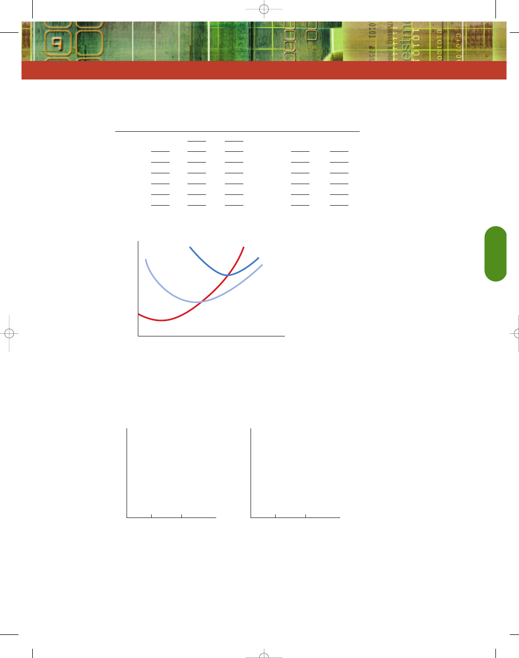
10. Complete the following table for a perfectly competitive firm, and indicate its profit-maximizing output.
Total Marginal
Total
Marginal
Total
Quantity
Price
Revenue
Revenue
Cost
Cost
Profit
6
10
30
3
30
7
35
8
42
9
51
10
62
11
75
12
90
11. Use the following diagram to answer a–d.
a. How much would a perfectly competitive firm produce at each of the indicated prices?
b. At which prices is the firm earning economic profits? Zero economic profits? Negative economic profits?
c. At which prices would the firm shut down?
d. Indicate what this firm’s supply curve would be.
12. Use the following diagram to answer a, b, and c.
a. Illustrate the relationship between a perfectly competitive firm’s demand curve and the market supply
and demand curve.
b. Illustrate the effects of an increase in market demand on a perfectly competitive firm’s demand curve.
c. Illustrate the effects of a decrease in market demand on a perfectly competitive firm’s demand curve.
Price
Quantity
100
200
0
Price
Quantity
100
200
0
Quantity (firm)
0
Price
P
3
P
2
P
1
P
0
MC
ATC
AVC
363
95469_13_Ch13_p331-364.qxd 29/12/06 12:45 PM Page 363
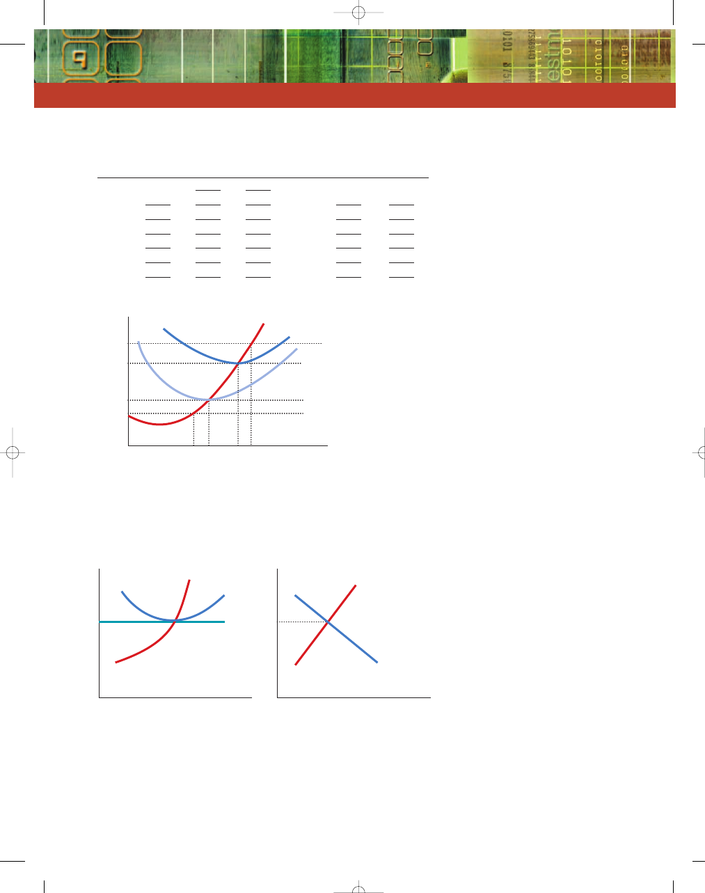
13. Complete the following table for a perfectly competitive firm, and indicate its profit-maximizing output.
Total Marginal
Total
Marginal
Total
Quantity
Price
Revenue
Revenue
Cost
Cost
Profit
6
10
30
3
30
7
35
8
42
9
51
10
62
11
75
12
90
14. Use the following diagram to answer a–d.
a. How much would a perfectly competitive firm produce at each of the indicated prices?
b. At which prices is the firm earning economic profits? Zero economic profits? Negative economic profits?
c. At which prices would the firm shut down?
d. Indicate what this firm’s supply curve would be.
15. Use the following diagrams to answer a and b.
a. Show the effect of an increase in demand on the perfectly competitive firm’s price, marginal revenue, output, and
profits in the short run.
b. Show the long-run effects of an increase in demand for the industry, and the effects on a perfectly competitive
firm’s price, marginal revenue, output, and profits for a constant-cost industry.
16. Describe what would happen to the industry supply curve and the economic profits of the firms in a competitive
industry if those firms were currently earning economic profits. What if they were currently earning economic losses?
MC
ATC
d
0
,
mr
0
D
0
S
0
Quantity (firm)
0
Price
Q
1
Q
3
Q
4
Q
0
Q
2
P
3
P
2
P
1
P
0
MC
ATC
AVC
364
95469_13_Ch13_p331-364.qxd 29/12/06 12:45 PM Page 364
Wyszukiwarka
Podobne podstrony:
Exploring Economics 4e Chapter 09
Exploring Economics 4e Chapter 18
Exploring Economics 3e Chapter 13
Exploring Economics 4e Chapter 30
Exploring Economics 4e Chapter 07
Exploring Economics 4e Chapter 11
Exploring Economics 4e Chapter 22
Exploring Economics 4e Chapter 17
Exploring Economics 4e Chapter 10
Exploring Economics 4e Chapter 14
Exploring Economics 4e Chapter 27
Exploring Economics 4e Chapter 25
Exploring Economics 4e Chapter 29
Exploring Economics 4e Chapter 15
Exploring Economics 4e Chapter 23
Exploring Economics 4e Chapter 31
Exploring Economics 4e Chapter 26
Exploring Economics 4e Chapter 24
Exploring Economics 4e Chapter 32
więcej podobnych podstron