
1
Taxes, Risk-Aversion, and the Size of the Underground Economy:
A Nonparametric Analysis With New Zealand Data
David E. A. Giles & Betty J. Johnson*
Department of Economics, University of Victoria
Victoria, B. C., V8W 2Y2, Canada
Revised, May 2000
Abstract:
We use nonparametric regression analysis to investigate the relationship between the effective tax
rate and the relative size of the underground economy, using New Zealand data. The underlying
theoretical framework is established, and it suggests an ambiguous prediction regarding the sign
of the relationship we are studying. However, our nonparametric empirical analysis, which also
allows for the non-stationarity of the time-series data, produces a positive and “S-shaped”
relationship, and this supports earlier empirical studies that imposed such functional forms. The
estimated model is used to simulate the effects of hypothetical tax changes on the size of the New
Zealand underground economy, and to draw policy conclusions.
* We would like to thank Greg Trandel for helpful correspondence, and Yehuda Kotowitz for
saving us from several mistakes. We are grateful to Judith Giles, Joseph Schaafsma, Gerald
Scully, John Small, Gugsa Werkneh and two referees for their very constructive comments on
earlier versions of this paper.
Keywords:
Tax evasion; underground economy; risk aversion, tax rates;
nonparametric regression.
JEL Classifications:
C14; C22; H26
Proposed Running Head:
Taxes and the Underground Economy
Contact Author:
Professor David Giles, Department of Economics, University of
Victoria, PO Box 1700, STN CSC, Victoria, BC, Canada, V8W 2Y2
FAX (250) 721-6214; Voice (250) 721-8540; e-mail
dgiles@uvic.ca

2
1. Introduction
There is a long-standing hypothesis that there is a relationship between taxes and the degree of
tax evasion, or the size of the “underground economy”. Various theoretical models have been
proposed in support of this hypothesis, but the associated empirical literature is relatively sparse.
In part this is due to the difficulty of obtaining meaningful time-series data for the size of the
underground workforce or underground output. In this paper, based on recent developments in
the theoretical literature on tax evasion, we examine in some detail the empirical relationship
between the relative size of the New Zealand underground economy and the effective tax rate in
that country, using annual time-series data for the period 1968 to 1994. The relative size of the
underground economy (UE) is measured as (UE/GDP), and the data are those generated by Giles
(1999) using a structural Multiple Indicator Multiple Causes (MIMIC) model. The (aggregate)
effective tax rate is defined as (TR/GDP), where TR is total tax revenue.
As is outlined below, there is theoretical justification for the hypothesis of a positive relationship
between the size of the underground economy and the tax rate, but this prediction is not readily
testable directly due to the form of the data that are generally available. In this paper we examine
the nature of this relationship empirically, making proper allowance for the non-stationarity of
our time-series data, and using nonparametric estimation in order to avoid distorting the
conclusions by “imposing” an assumed functional form on the analysis. Accordingly, this study
extends and corroborates that of Giles and Caragata (1999) and Caragata and Giles (2000) for
New Zealand - those authors adopted an explicit parametric analysis in their investigation of the
tax burden-underground economy relationship. Specifically, they considered various simple
polynomial and “S-shaped functions, and favoured a logistic functional form to “explain”
(UE/GDP) as a positive function of (TR/GDP).

3
Our objective here is to abstract from any such functional constraints, and to investigate some of
the practical implications of the recent theoretical model of Trandel and Snow (1999) by
estimating this relationship using nonparametric methods. Section 2 provides a general
theoretical background; and in Section 3 we re-formulate certain implications of the Trandel-
Snow model in terms of an hypothesis that can be tested empirically using macroeconomic data.
Section 4 discusses the available data, including issues of non-stationarity and possible
cointegration; and Section 5 deals with the estimation issues and results. Some of the economic
implications of the estimated model, including some simple simulation results, are described in
Section 6; and our concluding comments appear in Section 7.
2. Theoretical considerations
Schneider and Enste (1998) and Giles and Caragata (1999) discuss some of the previous
empirical evidence pertaining to the effect of taxes on the underground economy, stemming from
early contributions by Clotfelter (1983) and Crane and Nourzad (1987), to the more recent results
of Schneider (1994), Johnson et al. (1998), Cebula (1997), and Hill and Kabir (1996). This
evidence overwhelmingly supports the hypothesis of a positive relationship between taxes and the
size of the underground economy, though the data used and the details of the analysis vary
enormously from study to study.
Of primary interest here is the extensive theoretical literature that considers the role of taxes in
determining the size of the underground economy. In fact, much of this literature deals with
theoretical models that are quite narrow in their perspective. In particular, in the spirit of the
seminal contribution of Allingham and Sandmo (1972), much of this literature relates to models
of “pure tax evasion”. In such models, income is earned from only one source, and some of this
income is not declared to the taxation authority. Many of these models also assume that the

4
penalties for evasion are imposed as a fraction of undeclared income, rather than as a fraction of
the evaded tax, and/or that the tax system is linear
1
(e.g., Yitzhaki, 1974). Allowing for tax
progressivity and risk-averse tax-paying agents, the theoretical models of Pencavel (1979) and
Koskela (1983) predict that increasing the tax rate reduces the amount of tax evasion. However,
this result becomes ambiguous if flexibility is allowed with respect to labour’s hours worked, and
much of this literature is of questionable interest in terms of empirical verifiability.
On the other hand, there is also a more appealing theoretical literature relating to two-sector
“underground economy” models. In these models there are two sources of potential income, and
the probability that any evasion will be detected by the authorities differs between the two
sectors. In one sector, all earned income is “visible” with respect to taxation liability, while in the
other sector the possibility of tax evasion results in lower before-tax wages. Examples of such
contributions are those of Watson (1985), Kesselman (1989) and Trandel and Snow (1999).
Moreover, the latter model assumes that penalties for detected evasion are imposed in proportion
to the amount of evaded tax, which is exactly the situation in practice in most Western countries
(including New Zealand). Such “underground economy models” more relevant than “pure tax
evasion models” from an empirical viewpoint, as their underlying assumptions more closely
match reality, and so they provide interesting testable hypotheses.
The form of these hypotheses is, however, rather complicated. For example, the sign of the
relationship between the tax rate and the degree of tax evasion depends on what is assumed about
agents’ risk aversion. Trandel and Snow (1999) illustrate this. If taxes are progressive and if the
agents’ preferences exhibit decreasing absolute risk aversion, and non-decreasing relative risk
aversion, then their model predicts a positive relationship between the tax rate and the share of
the total labour force in the evasive sector of the economy. A positive relationship is also

5
predicted between the degree of tax-progressivity and the relative size of the underground labour
force. We examine aspects of the Trandel-Snow model in our own empirical analysis.
3. Formulating a testable hypothesis
In practice, aggregate data on the size of the underground economy are estimated in terms of the
value of “hidden” output, rather than the size of the associated labour force. Also, to facilitate
international comparisons, these figures are usually reported as a percentage of measured GDP.
For example, see Schneider and Enste (1998) for some extensive cross-country comparisons, and
Giles (1999) for a complete and recent time-series for the New Zealand underground economy.
This form of the data necessitates some manipulations of the predictions of the Trandel-Snow
model before they can be tested empirically.
This model is presented briefly in the Appendix. Of course, although its two-sector nature, and
the way in which it accounts for evasion penalties, match the New Zealand situation well, the
more detailed institutional characteristics of that country’s taxation system
2
render this theoretical
model somewhat stylized. This is a common situation, of course. However, the quality
3
of the
underground economy data, and the fact that they were generated without the use of effective tax
rate information (so that the modelling of a relationship between this rate and the underground
economy is not a spurious exercise), imply that the New Zealand situation provides a useful basis
for testing some of the implications of the Trandel-Snow model
4
empirically.
Within the framework given in the Appendix, Trandel and Snow prove that if agents’ preferences
exhibit decreasing absolute, and non-decreasing relative, risk aversion, then the size of the
underground economy (measured in employment terms) grows with the value of the marginal tax
rate that is faced in both sectors. Of course, as these preferences are not observable, but are

6
merely revealed through the agents’ actions, the sign of the relationship between the marginal tax
rate and the employment-size of the underground economy is itself effectively an empirical issue.
We now extend their analysis by reinterpreting this prediction in terms of average tax rates
(which differ between the evading and non-evading sectors), as well as in aggregate income (or
output) terms, rather than in employment terms. These extensions are important, empirically. Our
first task is to show that, as one would anticipate, the model predicts that the underground
economy grows with either an increase in the average tax rate in the non-evading sector, or with a
decrease in the (expected) average tax rate in the evading sector.
Proposition 1. Suppose that a fixed, non-zero, range of income is untaxed, that preferences
exhibit decreasing absolute and non-decreasing relative risk aversion, and that tax evasion is a
better-than-fair gamble. Then the size of the underground economy rises, if either the average
tax rate in the non-evading sector increases, or if the (expected) average tax rate in the evading
sector falls.
Proof. First, consider the non-evading sector. Using the notation in the Appendix, let f
n
(a*) =
τ
n
- t[y
n
(a*) – b] / y
n
(a*) = 0. By the implicit function theorem, (
∂
a*/
∂τ
n
) = - [(
∂
f
n
/
∂τ
n
) / (
∂
f
n
/
∂
a*)].
Now, (
∂
f
n
/
∂τ
n
) = 1, and (
∂
f
n
/
∂
a*) = - [tby'
n
(a*) / y
n
(a*)
2
]. So, (
∂
a*/
∂τ
n
) = [y
n
(a*)]
2
/ [tby'
n
(a*)] >
0, because y'
n
(a) > 0.
In the evading sector, let f
e
(a*) =
τ
e
- t{y
e
(a*) - b - [1 - p(1 + m)]x*} / y
e
(a*) = 0. Again, by the
implicit function theorem, (
∂
a*/
∂τ
e
) = - [(
∂
f
e
/
∂τ
e
) / (
∂
f
e
/
∂
a*)]. In this case, (
∂
f
e
/
∂τ
e
) = 1, and
(
∂
f
e
/
∂
a*) = - [tby'
e
(a*)] / [y
e
(a*)]
2
- [t{1 - p(1 + m)}x*y'
e
(a*)] / [y
e
(a*)]
2
. As y'
e
(a) < 0, it follows

7
that (
∂
a*/
∂τ
e
) <0 provided that [1 - p(1 + m)] > 0. This last condition is simply (1 - p) > pm,
which holds if tax evasion is a better-than-fair gamble.
•
Now consider the implications of the model in terms of hidden output, rather than hidden labour.
If ‘N’ is the size of the total labour force, then total declared (and measured) equilibrium gross
income in the non-evading sector is [N(1 - a*)y
n
]. In the evading sector, declared equilibrium
income is [Na*(y
e
- x*)], which equals measured gross income in that sector if evasion is not
detected. In the event of detection, measured income from this sector
5
will be [Na*y
e
]. Similarly,
equilibrium evaded income will be [Na*x*] in the absence of detection, and otherwise it will be
zero. So, the expected relative size
6
of the underground economy in aggregate income (output)
terms is:
u = [(1 - p)a*x*] / [(1 - a*)y
n
+ a*(y
e
- x*)].
(1)
Proposition 2. When a fixed, non-zero, range of income is untaxed and preferences exhibit
decreasing absolute and non-decreasing relative risk aversion, an increase in the marginal tax
rate may either increase or decrease the expected relative size of the underground economy,
measured in income terms.
Proof. Denoting (
∂
a*/
∂
t) by a*', and (
∂
x*/
∂
t) by x*', it follows from (1) that:
(
∂
u/
∂
t) = (1 - p){A(a*x*' + x*a*') - Ba*x*}/ A
2
,
(2)
where
A = [(1 - a*) y
n
+ a*( y
e
- x*)] ,
and
B = [(1 - a*)(
∂
y
n
/
∂
t) + a*' (y
e
- x* - y
n
) + a*{(
∂
y
e
/
∂
t) - x*'}].

8
Now, A > 0. Also, under the stated conditions, a*' > 0, so (
∂
y
n
/
∂
t) > 0, and (
∂
y
e
/
∂
t) < 0, by the
chain rule
7
. Clearly, from (2), regardless of the sign of x*', the sign of (
∂
u/
∂
t) is ambiguous.
•
So, perhaps not surprisingly, the nature of the effect of a change in the marginal tax rate on the
expected relative size of the underground economy is an empirical issue. It also follows from the
definitions of the average tax rates
(
τ
n
and
τ
e
), that a similar ambiguity arises with respect to the
signs of (
∂
u/
∂τ
n
) and (
∂
u/
∂τ
e
). The model does not provide a strong prediction of these effects.
So, in modelling the relationship between the macroeconomic aggregates (UE/GDP) and
(TR/GDP), the Trandel-Snow model does not predict the sign of the partial derivative, and this
issue is an empirical one. Their model and its predecessors are also, of course, silent on the
matter of the functional form of any such relationship between the tax rate and tax evasion. This
underscores the relevance of exploring a nonparametric approach in our empirical analysis below,
notwithstanding the fact that we have only a relatively small sample of data.
4. Data Issues
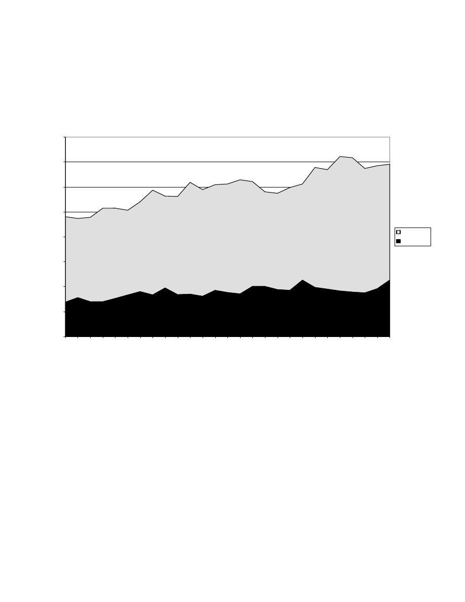
As noted already, we use two aggregate ratios, (UE/GDP) and (TR/GDP). Annual data for the
period 1968 to 1994 for the former variable are taken from Giles (1999), while the latter data are
compiled from official data released by Statistics New Zealand and Revenue New Zealand. Both
series are available on the web at www.uvic.ca/econ/uedata.html, and are displayed
8
in Figure 1.
As can be seen from the results in Table 1, we have tested each series for non-stationarity,
allowing for the possibilities of I(2), I(1) or I(0) data. We have used both the “augmented”
Dickey-Fuller (ADF) tests, in which the null hypothesis is non-stationarity, as well as the tests of
Kwiatowski et al. (KPSS) (1993) in which the null hypothesis is stationarity of the data. A 10%

9
significance level has been adopted to deal with the well-known low powers of these tests,
although the results are not sensitive to this choice.
In the case of the ADF tests, the augmentation level (p) has been chosen by the default method in
the SHAZAM (1997) package, as Dods and Giles (1995) show that this approach leads to low
size-distortion in the presence of moving-average errors with samples of the size being used here.
We have followed the sequential strategy of Dolado et al. (1990) to deal with the issue of the
inclusion/exclusion of drift and trend terms in the Dickey-Fuller regressions. So, in Table 1, t
dt
denotes the ADF unit root “t-test” with drift and trend terms included in the fitted regression; F
ut
is the corresponding ADF “F-test” for a unit root and zero trend; t
d
is the unit root “t-test” with a
drift but no trend in the fitted regression; F
ud
is the corresponding “F-test” for a unit root and a
zero drift; and t is the ADF unit root test when the fitted regression has no drift or trend term
included. Finite-sample critical values for our “t-tests” come from MacKinnon (1991), and those
for the “F-tests” are given by Dickey and Fuller (1979, 1981).
In the case of the KPSS tests, where the null is stationarity, and the alternative hypothesis is non-
stationarity, we have used both a zero value for the Bartlett window parameter, l, as well as l = 5.
The latter value is implied by the KPSS “l8 rule” for our sample size
9
. KPSS provide asymptotic
critical values for the test with null hypotheses of both level-stationarity and trend-stationarity.
Cheung et al. (1995) provide response-surface information that facilitates finite-sample critical
values in the trend-stationary case
10
.
The results in Table 1 indicate that both (UE/GDP) and (TR/GDP) are I(1), and hence are non-
stationary
11
. Accordingly, it is meaningful to test for possible cointegration between the two
series, and in Table 2 we show the results of applying the cointegrating regression ADF
(CRADF) test, in which the null is “no cointegration”, using MacKinnon’s (1991) exact critical

10
values. We see that there is modest evidence of cointegration at the 10% significance level.
Johansen’s (1988) likelihood ratio “trace test” was also used to test the null of no cointegration in
the context of a bivariate VAR model. With respect to the inclusion of drift and/or trend terms in
the the cointegating equations and/or the fitted VAR’s, the five possibilities suggested by
Johansen (1995) were all considered. Asymptotic critical values are given by Osterwald-Lenum
(1992), and in the usual case where one allows for a drift (but no trend) in both the data and the
cointegrating equations, a finite-sample correction to the critical values is suggested by Cheung
and Lai (1993). Using the usual information criteria we arrived at a lag length of k=4 for the VAR
models associated with the testing. We see that we clearly reject the null of zero cointegrating
vectors, but cannot reject the null of one cointegrating vector. Finally, we have used the
Leybourne-McCabe (1994) test, in which the null is “cointegration”. We generated finite-sample
critical values for this test by Monte Carlo simulation, using the experimental design described by
Leybourne and McCabe (1994, p.98), and SHAZAM (1998) code. Leybourne and McCabe’s
(1994, p.101) critical values for T=500 were reproduced exactly. We clearly cannot reject the null
of cointegration at any reasonable significance level
12
.
We have also tested for causality between (UE/GDP) and (TR/GDP), using the Toda-Yamamoto
(1995) approach, and the results
13
are summarised in Table 2. There is evidence of causality from
the latter variable to the former one, but only limited evidence of reverse causality. Taken in the
context of the theoretical discussion above, this supports an empirical model with (UE/GDP) as
the dependent variable.
5. Nonparametric estimation
In view of the above cointegration results, we may legitimately model the long-run relationship
between (UE/GDP) and (TR/GDP) by using the “levels” of these two ratio variables. No

11
differencing of the data is needed. As another option, we could construct an error-correction
model, which would be appropriate if we were interested in the short-run dynamics of the
relationship. Consistent with the theoretical literature, our estimation deals only with the first of
these possibilities.
Giles and Caragata (2000) considered some simple polynomial and Fourier series models of the
relationship between (UE/GDP) and (TR/GDP), before focussing on several “S-shaped”
functional forms such as the Gompertz, cumulative Normal, extreme-value, and logistic models.
The last of these was preferred by those authors in terms of overall data “fit” and statistical
significance. Before proceeding further, let us briefly elaborate on some aspects of these non-
linear parametric results. Fitting an OLS cubic relationship between these variables results in
totally insignificant parameter estimates. A quadratic model generates reasonably significant
parameter estimates with a Durbin-Watson statistic of 1.53, and with DeBenedictis-Giles (1998)
FRESET test results that strongly indicate no mis-specification. The latter model is, of course,
extremely restrictive in terms of the curvature properties that it can capture. The parameter
estimates imply a positive but decreasing relationship between the underground economy ratio
and the tax rate for values of the latter less than about 33%. At the latter value there is a turning
point in the relationship. A simple linear relationship was inadequate whether OLS or
instrumental variables estimation was adopted
14
.
We have also explored the Giles and Caragata (2000) results further by conducting a series of
Davidson and MacKinnon (1981) “J-tests” to discriminate between the polynomial models and
their preferred logistic model, these models being “non-nested”. These tests suggest the rejection
of the logistic model against linear, quadratic, and cubic alternatives. However, they also suggest
the rejection of the linear and quadratic models against the logistic model. The unsatisfactory
nature of the cubic results has been noted already.

12
These inconclusive results support the use of a flexible nonparametric approach to estimating this
relationship, and our model takes the simple form:
(UE/GDP)
t
= m{(TR/GDP)
t
} +
ε
t
,
(3)
(3)
where the function “m” is the conditional mean of the dependent variable and the
ε
t
’s
are Normal,
independent and homoskedastic.
In (3), the data for the dependent variable have been estimated by Giles (1999) using MIMIC
model analysis. That is, the dependent variable is random for reasons other than that allowed for
with the inclusion of the usual error term in the model. In fact, this causes no problem for the
properties of our estimates, or their interpretation. This additional source of randomness can be
assumed to be independent of
ε
τ
,
and our nonparametric estimator will be consistent, anyway,
under very weak conditions.
Estimation of (3) was undertaken with the NONPAR routine in the SHAZAM (1997)
econometrics package, using the Nadaraya-Watson estimator with a Normal kernel, and the
bandwidth parameter was chosen by Silverman’s (1986, p.45) “optimal” method. Some
experimentation verified that the results were not particularly sensitive to the choice of kernel or
bandwidth. We also paid special attention to “edge effect” associated with nonparametric
regression, especially when the sample is relatively small. In particular, we re-estimated our
nonparametric model using Rice’s (1984) boundary modified estimator, with a range of values for
his “
ρ
” parameter. We found that the results reported below were quite insensitive to this
refinement, unless “
ρ
” is close to its minimum value of zero. Even in this case the general non-

13
linear shape of the estimated relationship between (UE/GDP) and (TR/GDP) was not affected.
This robustness of the results is encouraging, especially given that our nonparametric estimation
is based on quite a small-sized sample.
We also considered versions of (3) that included the
growth of real GDP, and/or one-period or two-period lagged values of (UE/GDP) or (TR/GDP) as
additional explanatory variables. However, none of these were supported by the usual
information criteria, and our preferred simple estimates are given in Table 3. The LM tests for
autocorrelation have their usual asymptotic interpretation
15
, and are generally quite satisfactory.
The FRESETS results support the form of the estimated model when interpreted in terms of the
associated information measures.
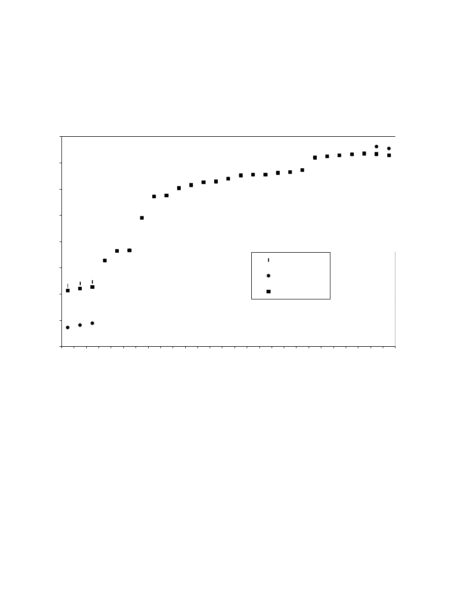
The estimated model’s within-sample “predictions”, with the (TR/GDP) variable sorted into
ascending order, appear in Figure 2. The general shape of this relationship supports the earlier
use of a logistic function by Giles and Caragata (1999) and by Caragata and Giles (2000). Also
shown in Figure 2, for comparative purposes, are the predictions corresponding to the use of
Rice’s (1984) estimator, with two different choices of his “
ρ
”. Interestingly, the slight downturn
in the fitted relationship at historically high tax rates is consistent with the curvature result noted
above with respect to a naive quadratic model.
Table 4 shows the corresponding predicted values for (UE/GDP), together with lower and upper
limits for the corresponding 95% prediction interval, and the estimated elasticities. The
predictions range in value from 7.52% to 9.51% of GDP. These values should be compared with
the “actual” sample values for (UE/GDP) given by Giles (1999), which range from 6.84% to
11.31%.

14
6. Further economic implications
The corresponding estimated elasticities between the effective tax rate and the (UE/GDP) ratio
also appear in Table 4. As these two variables are already expressed in percentage terms, these
elasticities must be interpreted with care. For example, 1986 was an interesting year in the
history of New Zealand taxation policy, with the introduction of the Goods and Services Tax
(GST) in October, and the simultaneous major changes to sales taxes and to the personal income
tax and corporate income tax schedules
16
. In 1986 the effective tax rate was 29.85% and the
estimated underground economy elasticity was 0.303. This implies that a 10% cut in the effective
tax rate would lead (with some unspecified delay) to a 3.03% drop in the %(UE/GDP). A 10%
cut in the effective tax rate means reducing it from 29.85% to 26.87%. The %(UE/GDP) in New
Zealand in 1986 was 9.23%. So, it is predicted that the size of the underground economy would
have dropped by 3.03% (that is, it would have dropped from 9.23% of GDP to 8.95% of GDP) to
reach a new equilibrium
17
had the tax burden been reduced by 10% in that year, without any
change in the “tax-mix”. Of course, as this analysis is based on a cointegrating relationship, the
above discussion sheds no light on the speed of this adjustment to the new equilibrium position.
In Table 5 we see the results of “simulating” the estimated relationship in (3) to get predicted
values for (UE/GDP) as the effective tax rate ranges hypothetically in value from 17% to 38%. It
is especially interesting to note that as the tax rate is decreased, the effect on the underground
economy begins to “flattens out” at a tax rate below 25%. Although nonparametric estimation
does not allow us to extrapolate below the range of our sample data, this observation accords
remarkably well with the conclusions of Caragata and Giles (2000) and of Scully (1996). Using
the criterion of maximizing the responsiveness of the underground economy to tax rate changes,
the former authors concluded that the “optimal” effective tax rate is approximately 21%. Scully’s
results suggested a growth-maximizing effective tax rate of 20% in the case of New Zealand.

15
Interestingly, therefore, there is a close consistency between the tax rate that needs to be targeted
from an economic growth viewpoint, and the one that needs to be targeted from a compliance
viewpoint.
7. Conclusions
In this paper we have used nonparametric time-series regression to examine some of the
predictions of a class of theoretical models of the underground economy. In particular, we have
interpreted the recent model of Trandel and Snow (1999) in aggregate terms, and have provided
empirical evidence concerning the partial relationship between the relative (output) size of the
underground economy and the effective tax rate, using New Zealand data. This theoretical model
predicts an ambiguous sign for the above relationship, but empirically we find a positive, “S-
shaped” relationship that fits the data well over our sample period, 1968 to 1994.
When we simulate the model over a plausible range of tax rate values we obtain results that
accord closely with other related results by Caragata and Giles (2000) and Scully (1996), each of
whom address the issue of an “optimal effective tax rate” for New Zealand from different
perspectives. In particular, our nonparametric model suggests that the responsiveness of the
underground economy to simple changes in the tax burden drops markedly when the effective tax
rate drops below about 25%.
The possibility that the adjustment of the underground economy to changes in the tax burden is
asymmetric (in the upward and downward directions) is an important issue that is not explored
here. This is discussed in the New Zealand context by Giles et al. (1999). The authors are also
analyzing such asymmetry issues in the context of the Canadian underground economy data
derived by Giles and Tedds (2000).

16
Appendix – The Trandel and Snow Model
There are two sectors, workers are identical, and each supplies a unit of labour either to sector ‘e’
(or to sector ‘n’), in which evasion is (or is not) undertaken. Income per worker in sector ‘i’ is
denoted ‘y
i
’; ‘a’ is the share of the workforce in sector ‘e’; and ‘t’ is the constant marginal tax rate
(above a positive threshold level of income, ‘b’). Faced with a probability ‘p’ that evaded income
will be detected, and penalised in proportion (m) to the additional tax owed, workers in the
evading sector choose a level of undeclared income, ‘x’, to maximise expected utility:
(1 – p)U[y
e
(1 – t) + bt + xt] + pU[y
e
(1 – t) + bt – mxt].
(A.1)
As labour is mobile, an equilibrium is achieved by finding optimal a* and x* values to equate the
expected utility of working in each sector. This requires:
U[y
n
(a*)(1 – t) + bt] = (1 – p)U[y
e
(a*)(1 – t) + bt + x*t] + pU[y
e
(a*)(1 – t) + bt – mx*t]. (A.2)
Assuming that workers’ preferences exhibit decreasing absolute and non-decreasing relative, risk
aversion, (A.2) is used by Trandel and Snow to establish several results relating the (labour) size
of the underground economy to changes in the marginal tax rate, and in tax progressivity.
To derive our results in section 3, we use the fact that the (actual) average tax rate faced by
workers in the non-evading sector is
τ
n
= t [y
n
(a*) – b] / y
n
(a*). Similarly the (expected) average
tax rate in the evading sector is
τ
e
= t { y
e
(a
*
) – b – [1 – p(1 + m)]x*} / y
e
(a*). As Trandel and
Snow (1999; p 221) note,
τ
n
>
τ
e
. This is because for tax evasion is to be a better-than-fair
gamble, we require (1 – p) > pm.

17
References
Allingham, M. G. and Sandmo, A. (1972) “Income tax evasion: a theoretical analysis”, Journal
of Public Economics 1, 323-338.
Caragata, P. J. and D. E. A. Giles (2000) “Simulating the relationship between the hidden
economy and the tax level and tax mix in New Zealand”, in G. W. Scully and P. J.
Caragata (eds.), Taxation and the Limits of Government, Boston: Kluwer, 221-240.
Cebula, R. J. (1997) “An empirical analysis of the impact of government tax and auditing
policies on the size of the underground economy: the case of the United States, 1993-94”,
American Journal of Economics and Sociology 56, 173-185.
Cheung, Y-W. and K. S. Lai (1993), “Finite-sample sizes of Johansen’s likelihood ratio tests
for cointegration”, Oxford Bulletin of Economics and Statistics, 55, 313-328.
Cheung, Y-W., M. D. Chinn and T. Tran (1995) “How sensitive are trends to data definitions?
Results for East Asian countries”, Applied Economics Letters 2, 1-6.
Clotfelter, C. T. (1983) “Tax evasion and tax rates: an analysis of individual returns”, Review of
Economics and Statistics 65, 363-373.
Crane, S. E. and F. Norzad (1987) “On the treatment of income tax rates in empirical analysis of
tax evasion” Kyklos, 40, 338-348.
Davidson, R. and J. MacKinnon (1981) “Several tests for model specification in the presence of
alternative hypotheses”, Econometrica, 49, 781-793.
DeBenedictis, L. F. and D. E. A. Giles (1998) “Diagnostic testing in econometrics: variable
addition, RESET, and Fourier approximations”, in A. Ullah & D. E. A. Giles (eds.),
Handbook of Applied Economic Statistics, New York: Marcel Dekker, 383-417.
DeBenedictis, L. F. and D. E. A. Giles (2000) “Robust specification testing in regression: the
FRESET test and autocorrelated errors”, Journal of Quantitative Economics, to appear.

18
Dickey, D. A. and W. A. Fuller (1979) “Distribution of the estimators for autoregressive time
series with a unit root”, Journal of the American Statistical Association 74, 427-431.
Dickey, D. A. and W. A. Fuller (1981) “Likelihood ratio statistics for autoregressive time series
with a unit root”, Econometrica 49, 1057-1072.
Dods, J. L. and D. E. A. Giles (1995) “Alternative strategies for ‘augmenting’ the Dickey-Fuller
test: size-robustness in the face of pre-testing”, Journal of Statistical Computation and
Simulation 53, 243-258.
Dolado, J. J., T. Jenkinson and S. Sosvilla-Rivero (1990) “Cointegration and unit roots”, Journal
of Economic Surveys 4, 249-273.
Giles, D. E. A. (1997) “Causality between the measured and underground economies in New
Zealand”, Applied Economics Letters 4, 63-67.
Giles, D. E. A. (1999) “Modelling the hidden economy and the tax-gap in New Zealand”,
Empirical Economics 24, 621-640.
Giles, D. E. A. (2000) “Modelling the tax compliance profiles of New Zealand firms: evidence
from audit records”, in G.W. Scully and P.J. Caragata (eds.), Taxation and the Limits of
Government, Boston: Kluwer, 243-269.
Giles, D. E. A. and P. J. Caragata (1999) “The learning path of the hidden economy: the tax
burden and tax evasion in New Zealand”, Econometrics Working Paper EWP9904,
revised, Department of Economics, University of Victoria, and forthcoming in Applied
Economics.
Giles, D. E. A. and L. M. Tedds (2000) Taxes and the Canadian Underground Economy,
Toronto: Canadian Tax Foundation, in press.
Giles, D. E. A., G. T. Werkneh, and B. J. Johnson (1999) “Asymmetric responses of the
underground economy to tax changes: evidence from New Zealand data”, Econometrics
Working Paper, EWP9911, Department of Economics, University of Victoria.
Hardle, W. (1990) Applied Nonparametric Regression, Cambridge: Cambridge University Press.

19
Hill, R. and M. Kabir (1996) “Tax rates, the tax mix, and the growth of the underground
economy in Canada: what can we infer?”, Canadian Tax Journal 44, 1552-1583.
Johansen, S. (1988), “Statistical analysis of cointegration vectors,” Journal of Economic
Dynamics and Control, 12, 231-254.
Johansen, S. (1995), Likelihood-Based Inference in Cointegrated Vector Autoregressive Models,
Oxford, Oxford University Press.
Johnson, B. J. (1998) “Money-income causality and the New Zealand underground economy”,
M.A. Extended Essay, Department of Economics, University of Victoria.
Johnson, S., D. Kaufmann and P. Zoido-Lobaton (1998) “Regulatory discretion and the
unofficial economy”, American Economic Review 88, 387-392.
Kesselman, J. R. (1989) “Income tax evasion: an intersectoral analysis”, Journal of Public
Economics 38, 137-182.
Koskela, E. (1983) “A note on progression, penalty schemes and tax evasion”, Journal of Public
Economics 22, 127-133.
Kwiatowski, D., P. C. B. Phillips, P. Schmidt, and Y. Shin (1992) “Testing the null hypothesis
of stationarity against the alternative of a unit root: how sure are we that economic time
series have a unit root?”, Journal of Econometrics 54, 159-178.
Leybourne, S. J. and B. P. M. McCabe (1994) “A simple test for cointegration”, Oxford Bulletin
of Economics and Statistics 56, 97-103.
MacKinnon, J. G. (1991) “Critical values for co-integration tests”, in R. F. Engle and C. W. J.
Granger (eds.), Long-Run Economic Relationships, Cambridge: Cambridge University
Press, 267-276.
Osterwald-Lenum, M. (1992), “A note with quantiles of the asymptotic distribution of the
maximum likelihood cointegration rank Test statistics”, Oxford Bulletin of Economics
and Statistics, 54, 461-472.

20
Pencavel, J. H. (1979) “A note on income tax evasion, labor supply, and nonlinear tax
schedules”, Journal of Public Economics 12, 115-124.
Rice, J. (1984) “Bandwidth choice for nonparametric kernel regressions”, Annals of Statistics 12,
1215-1230.
Robinson, P. M. (1997), “Large-sample inference for nonparametric regression with dependent
errors”, Annals of Statistics, 25, 2054-2083.
Schneider, F. (1994) “Can the shadow economy be reduced through major tax reforms? An
empirical investigation for Austria”, supplement to Public Finance 49, 137-152.
Schneider, F. and D. Enste (1998) “Increasing shadow economies all over the world – fiction or
reality? A survey of the global evidence of their size and their impact from 1970 to
1995”, Arbeitspapier 9819, Department of Economics,University of Linz, and
forthcoming in Journal of Economic Literature.
Scully, G. W. (1996) “Taxation and economic growth in New Zealand”, Pacific Economic
Review 1, 169-177.
SHAZAM (1997) SHAZAM Econometrics Package, User's Guide, Version 8.0, New York:
McGraw-Hill.
Silverman, B. W. (1986) Density Estimation, London: Chapman and Hall.
Toda, H. Y. and T. Yamamoto (1995) “Statistical inference in vector autoregressions with
possibly integrated processes”, Journal of Econometrics 66, 225-250.
Trandel, G. and A. Snow (1999) “Progressive income taxation and the underground economy”,
Economics Letters, 62 217-222.
Watson, H. (1985) “Tax evasion and labor markets”, Journal of Public Finance 27, 231-246.
Yitzhaki, S. (1974) “A note on income tax evasion: a theoretical analysis”, Journal of Public
Economics 3, 201-202.

21
Footnotes
1. A “linear” tax system is one in which the tax rate is a fixed proportion of income - it is a
“flat tax” system with a zero exemption-threshold. If the tax system is linear then any
fraction of undeclared income can also be represented as a fraction of evaded tax.
2. The tax schedule in New Zealand was simplified considerably during our sample period.
With respect to corporate taxes, the tax structure assumed in the Trandel-Snow model is
closely approximated. In the case of personal income taxes the statutory rate is certainly
progressive, with a very simple scale (in recent years), but with a zero “threshold” level.
3. The accuracy of Giles’ (1999) aggregate time-series measure of the underground
economy in New Zealand is supported by the independent micro-evidence, based on
Revenue New Zealand business audit records, discussed by Giles (2000).
4. Figure 1 shows that our data exhibit considerable cyclical variation over our sample,
implying that our analysis is based on “informative” empirical evidence.
5. The penalty for evasion is not counted as part of generated “income”, but this does not
affect the conclusions below.
6. We are considering the expected value of the ratio of underground to measured income.
Alternatively, one could consider the ratio of expected underground income to expected
measured income. Pursuing this alternative yields the same implications as below.
7. Recall that y'
n
(a) > 0 and y'
e
(a) < 0.
8. GDP is conventional “measured” GDP. This is a standard way of defining the effective
tax rate, and it makes the UE measure comparable to other international series. Some
countries (not including New Zealand) are considering “adjusting” GDP for underground
activity, so an alternative would be to use UE/(GDP+UE). This was not pursued, as UE
incorporates a mixture of both “legally-based” and “illegally-based” underground
activity, and only the former is relevant to the measurement of GDP.

22
9. This rule sets l = INT [8(T/100)
1/4
].
10. For our sample size the asymptotic and finite-sample KPSS critical values are very
similar, so the unavailability of the latter in the case of a level-stationary null should not
be of concern.
11. We also tested the logarithms of the two variables for unit roots, and found log(UE/GDP)
to be I(0) and log(TR/GDP) to be I(1). So, there can be no cointegration between these
two variables, and it would be inappropriate to model the relationship between them
without differencing the latter variable. We have not pursued this possibility here.
12. The tests for cointegration are actually tests for a linear cointegrating relationship
between (UE/GDP) and (TR/GDP). In our case, the OLS residuals from this
cointegrating regression suggest that a non-linear relationship may also be worth
investigating. (The Durbin-Watson statistic is 1.280, with an exact p-value of 0.015; the
LM tests for fifth-order and sixth-order autocorrelation are significant at the 1% level.
The RESET and FRESET tests are generally satisfactory, but the FRESETS(3) statistic is
2.588, with a p-value of 0.053, and the RESET(2) statistic is 4.976, with a p-value of
0.035. The robustness of the FRESETS tests to error-term autocorrelation is documented
by DeBenedictis and Giles, 2000). This further supports our use of a nonparametric
specification below.
13. Taking account that the data are I(1), the testing was undertaken within a two-equation
VAR model, in which two “own” lagged variables and one “other” lagged variable
appeared as the regressors. The insignificant intercepts were suppressed. The Toda-
Yamamoto (1995) methodology ensures the asymptotic validity of the Wald test applied
to the one-period lagged value of the “other” variable here. This Wald statistic is just the
square of the usual “t-statistic” in this case.
14. As noted in footnote 12, the linear models we estimated exhibited mis-specification of the
functional form. In addition, the R
2
values were of the order of only 30%.

23
15. The asymptotic normality of kernel regression estimators (and associated statistics) is
well known. For example, see Hardle (1990, pp.99-100). Robinson (1997) shows that
asymptotic normality holds approximately even in the case of dependent errors.
16. Initially the GST was levied at a rate of 10%, wholesale taxes were abolished and the top
marginal personal income tax rate was reduced from 66% to 48%. Other major changes
to these rates have taken place subsequently.
17. Note that this is a drop of 3.03%, and not a drop of 3.03 percentage points.

24
Table 1. Unit root test results
a. Augmented Dickey-Fuller tests
a
T
p
t
dt
F
ut
t
d
F
ud
t
Outcome
UE/GDP
H
0
:
I(2)
23
2
-3.44
n.a.
n.a.
n.a.
n.a.
Reject I(2)
[H
A
:
I(1)]
H
0
:
I(1)
24
2
-2.70
3.66
-1.63
2.14
1.06
I(1)
[H
A
:
I(0)]
TR/GDP
H
0
:
I(2)
23
2
-2.62
3.43
-2.65
n.a.
n.a.
Reject I(2)
[H
A
:
I(1)]
H
0
:
I(1)
24
2
-2.42
3.21
-1.40
2.73
1.63
I(1)
[H
A
:
I(0)]
b. KPSS tests
b
T
Level-Stationary
Trend-Stationary
Outcome
l=0
l=5
l=0
l=5
UE/GDP
H
0
:
I(0)
27
1.519
0.520
0.131
0.110
I(1)
[H
A
:
I(1)]
TR/GDP
H
0
:
I(0)
27
0.099
0.073
0.129
0.081
I(1)
[H
A
:
I(1)]
Notes:
a.
The outcomes are based on finite-sample 10% critical values from MacKinnon (1991).
b. The outcomes are based on finite-sample 10% critical values from Cheung et al. (1995),
and the KPSS 10% asymptotic critical values.

25
Table 2. Cointegration and causality test results
a. Cointegrating regression augmented Dickey-Fuller “t-tests”
T
p
No Trend
Trend
Outcome
a
R
2
t
R
2
t
27
0
0.40
-3.434
0.58
-3.856
Cointegration
(-3.57)
(-4.15)
[-3.20]
[-3.77]
b. Johansen’s “trace” likelihood ratio tests
Drift/Trend Case
b
(1)
(2)
(3)
(4)
(5)
Trace Test Statistic, H
0
: Zero Cointegrating Vectors
27.32
32.02
22.88
31.26
30.38
Asy. 10% crit.
10.47
17.85
13.33
c
22.76
16.06
Asy. 5% crit.
12.53
19.96
15.41
c
25.32
18.17
Asy. 1% crit.
16.31
24.60
20.04
c
30.45
23.46
Trace Test Statistic, H
0
: No More Than One Cointegrating Vector
4.45
5.16
0.97
7.83
7.81
Asy. 10% crit.
2.86
7.52
2.69
d
10.49
2.57
Asy. 5% crit.
3.84
9.24
3.76
d
12.25
3.74
Asy. 1% crit.
6.52
12.97
6.65
d
16.26
6.40

26
Table 2. Cointegration and causality test results (continued)
c. Leybourne-McCabe cointegration tests
e
T
h
1
Asymptotic
Finite-Sample
Outcome
Critical Values
Critical Values
27
0.122
(0.31)
(0.35)
Cointegration
[0.23]
[0.25]
d. Granger causality tests
Causality
Wald Test
Asymptotic p-value
Bootstrapped p-value
f
(
χχ
2
(1))
(TR/GDP)
^
(UE/GDP)
3.594
5.8%
0.3%
(UE/GDP)
^
(TR/GDP)
3.664
5.6%
23.4%
Notes:
a.
MacKinnon’s (1991) finite-sample 5% (10%) critical values appear in parentheses
(brackets).
b.
(1) No drift/no trend in cointegrating equation or fitted VAR.
(2) Drift/no trend in cointegrating equation; no drift in fitted VAR.
(3) Drift/no trend in both cointegrating equation and fitted VAR.
(4) Drift and trend in cointegrating equation; no trend in fitted VAR.
(5) Drift and trend in both cointegrating equation and fitted VAR.
c. The corresponding finite-sample critical values are 20.13, 23.27 and 30.26 respectively.
d. The corresponding finite-sample critical values are 4.06, 5.67, and 10.04 respectively.
e. 5% (10%) critical values appear in parentheses (brackets).
f.
These are based on 5,000 bootstrap replications.

27
Table 3. Nonparametric estimation of the relationship between (UE/GDP) & (TR/GDP)
(Simple nonparametric regression)
Bandwidth Parameter
0.548
R
2
(Adjusted R
2
)
0.492
(0.428)
Cross-Validation Mean Square Error
0.794
AIC
(SC)
[FPE]
0.842
(1.016)
[0.844]
Residuals Analysis
Durbin-Watson Statistic
1.433
Runs Test, Normal Statistic (p-value)
-0.975
(0.330)
Coefficient of Skewness (Standard Deviation)
0.956
(0.448)
Coefficient of Excess Kurtosis (Standard Deviation)
0.665
(0.872)
Jarque-Bera, Chi-Square, asy.
χ
2
(2) (p-value)
3.681
(0.159)
Chi-Square Goodness of Fit, asy.
χ
2
(3) (p-value)
6.094
(0.107)
LM(1), asy. Standard Normal (p-value)
1.006
(0.157)
LM(2), asy. Standard Normal (p-value)
0.208
(0.418)
LM(3), asy. Standard Normal (p-value)
0.205
(0.419)
LM(4), asy. Standard Normal (p-value)
0.152
(0.440)
FRESETS(1)
a
: AIC (SC) [FPE]
0.995
(1.479)
[1.016]
FRESETS(2)
a
: AIC (SC) [FPE]
1.110
(2.086)
[1.215]
FRESETS(3)
a
: AIC (SC) [FPE]
1.330
(2.395)
[1.333]
Note:
a.
FRESETS(i) is the DeBenedictis and Giles (1998) Fourier version of the RESET test
with “i” sine and cosine terms. The test statistic
cannot be computed in the
nonparametric case, but the resulting information criteria that emerge when these extra
terms are added into the nonparametric regression can be compared with their
counterparts from the original model, given in the first part of this table. As the latter are
smaller than those for the FRESETS regressions, this suggests “no mis-specification”.

28
Table 4. Ranked nonparametric within-sample predictions and 95% confidence limits
Lower
Predicted
Upper
(TR/GDP)%
Elasticity
(UE/GDP)%
7.080
7.525
7.970
23.643
0.467
7.124
7.559
7.994
23.859
0.531
7.155
7.584
8.013
24.003
0.577
7.510
7.911
8.312
25.287
1.053
7.655
8.053
8.452
25.693
1.178
7.667
8.065
8.464
25.726
1.186
8.163
8.557
8.952
26.996
1.157
8.495
8.888
9.281
28.075
0.754
8.506
8.899
9.292
28.123
0.736
8.620
9.013
9.407
28.696
0.536
8.665
9.059
9.454
28.992
0.453
8.706
9.103
9.499
29.328
0.379
8.716
9.113
9.511
29.423
0.362
8.755
9.157
9.559
29.852
0.303
8.794
9.205
9.616
30.412
0.267
8.804
9.217
9.631
30.563
0.264
8.804
9.217
9.631
30.564
0.264
8.824
9.244
9.665
30.904
0.267
8.832
9.256
9.680
31.047
0.272
8.854
9.286
9.717
31.403
0.290
9.003
9.478
9.952
33.432
0.295
9.017
9.497
9.977
33.681
0.259
9.026
9.511
9.996
33.884
0.224
9.034
9.529
10.024
34.220
0.158
9.033
9.540
10.046
34.527
0.094
8.941
9.525
10.109
35.843
-0.167
8.908
9.513
10.119
36.080
-0.204

29
Table 5. Simulated values of (UE/GDP)% for various effective tax rates
(TR/GDP)
(UE/GDP)
(%)
(%)
Nonparametric
Logistic
17
7.314
6.519
18
7.307
6.668
19
7.306
6.821
20
7.312
6.977
21
7.331
7.136
22
7.370
7.299
23
7.445
7.465
24
7.584
7.634
25
7.821
7.808
26
8.170
7.984
27
8.559
8.164
28
8.870
8.348
29
9.060
8.536
30
9.171
8.728
31
9.252
8.923
32
9.340
9.122
33
9.438
9.326
34
9.518
9.533
35
9.545
9.745
36
9.517
9.960
37
9.451
10.180
38
9.367
10.405
30
Figure 1. Effective tax rate and underground economy, New Zealand 1968-1994
0
5
10
15
20
25
30
35
40
1968 1969 1970 1971 1972 1973 1974 1975 1976 1977 1978 1979 1980 1981 1982 1983 1984 1985 1986 1987 1988 1989 1990 1991 1992 1993 1994
Year
%
(TR/GDP)
(UE/GDP)
31
Figure 2. Non-parametric relationship between underground economy and effective tax rate: New
Zealand, 1968-1994
6.6
7.0
7.4
7.8
8.2
8.6
9.0
9.4
9.8
23.6
24.0
25.7
27.0
28.1
29.0
29.4
30.4
30.6
31.0
33.4
33.9
34.5
36.1
TR/GDP (%)
UE/GDP (%)
No Adjustment
Rho=0.1
Rho=0.9
Wyszukiwarka
Podobne podstrony:
nieparametryczne v2 prezentacja Nieznany
nieparametryczne v2 streszczeni Nieznany
nieparametryczne v1 artykul
panele v2 artykul
duration analysis v2 artykul
markov v2 artykul
DTC v2
testy nieparametryczne
dodatkowy artykul 2
ARTYKUL
Elektro (v2) poprawka
l1213 r iMiBM lakei v2
logika rozw zadan v2
więcej podobnych podstron