
Krzysztof Marzjan
Podstawowe problemy automatyki
2
Podstawowe problemy automatyki 4
ocena pracy UAR, ćwiczenia wspomagane MATLAB-em
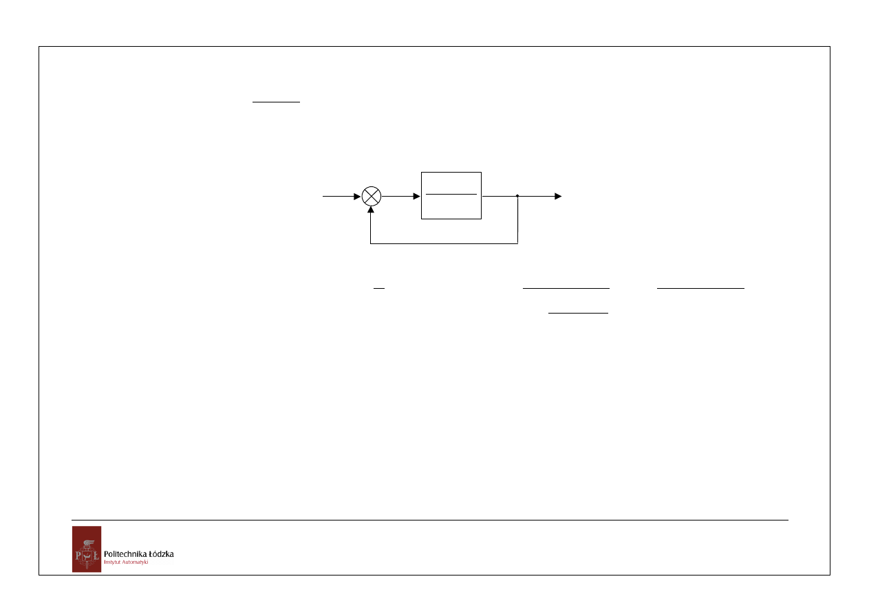
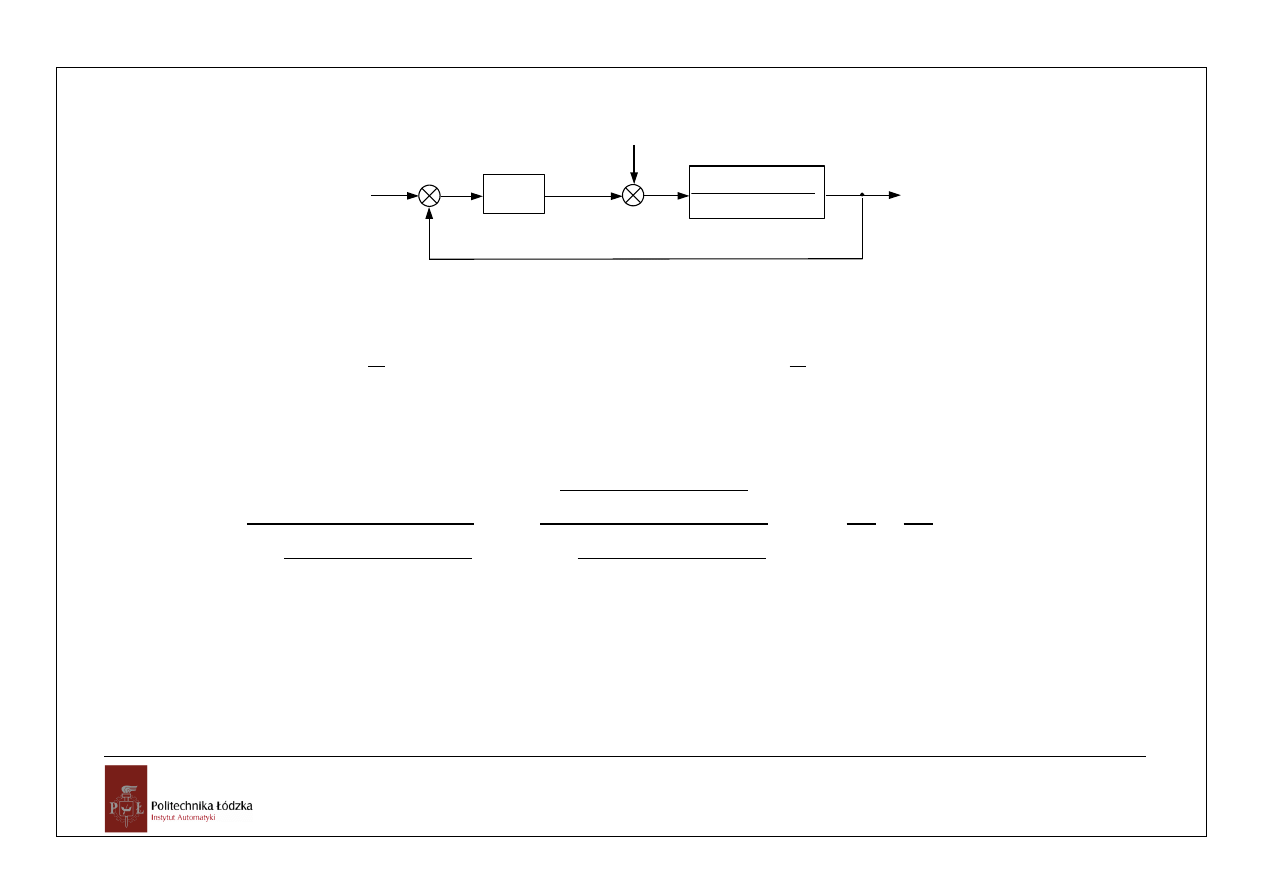
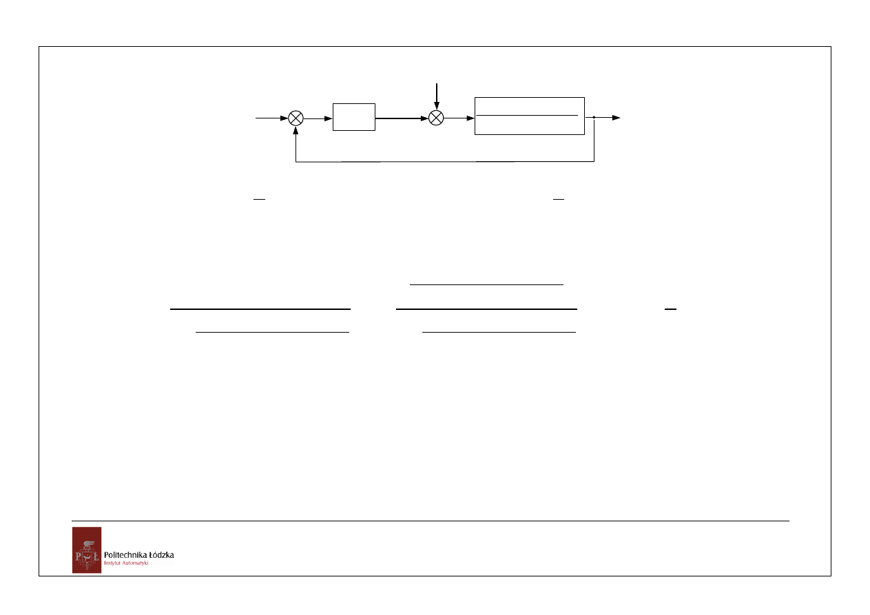
Problem 1.
Układ o transmitancji
)
1
(
2
)
(
s
s
s
G
odwiedziono sztywnym, ujemnym sprzężeniem zwrotnym. Czy układ ten jest
astatyczny pierwszego rzędu względem wymuszenia (uzasadnij)? Jaka jest wartość ustalona uchybu przy
wymuszeniu
)
(
1
2
)
(
t
t
t
u
i zerowych warunkach początkowych?
)
1
(
2
s
s
u(s)
y(s)
e(s)
_
Układ jest astatyczny względem wymuszenia, ponieważ:
0
2
)
1
(
)
1
(
)
1
(
2
1
1
)
(
1
)
(
)
(
)
(
)
(
0
0
0
0
0
s
s
s
s
lim
s
s
lim
s
G
lim
s
s
sG
lim
s
se
lim
t
e
lim
e
s
s
e
s
e
s
s
t
3
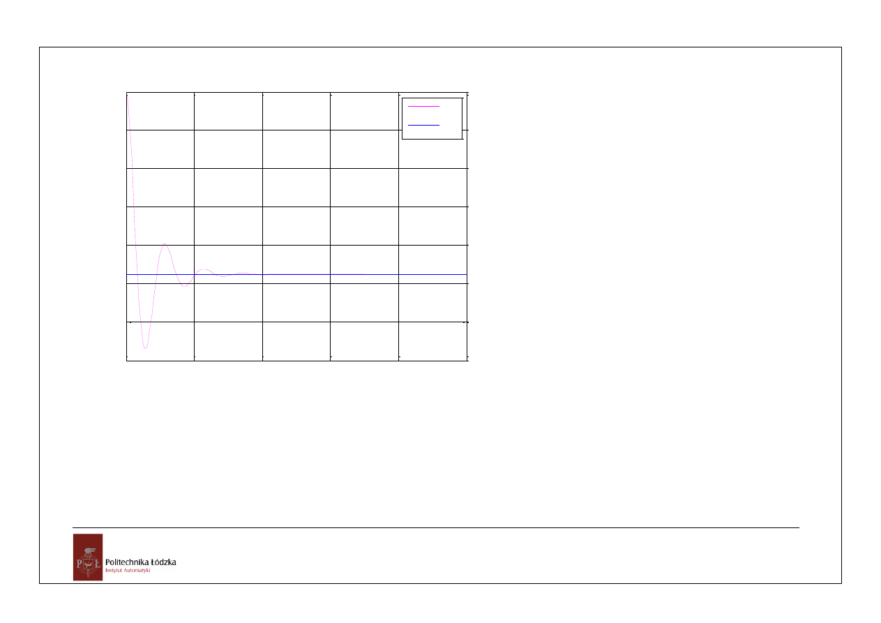
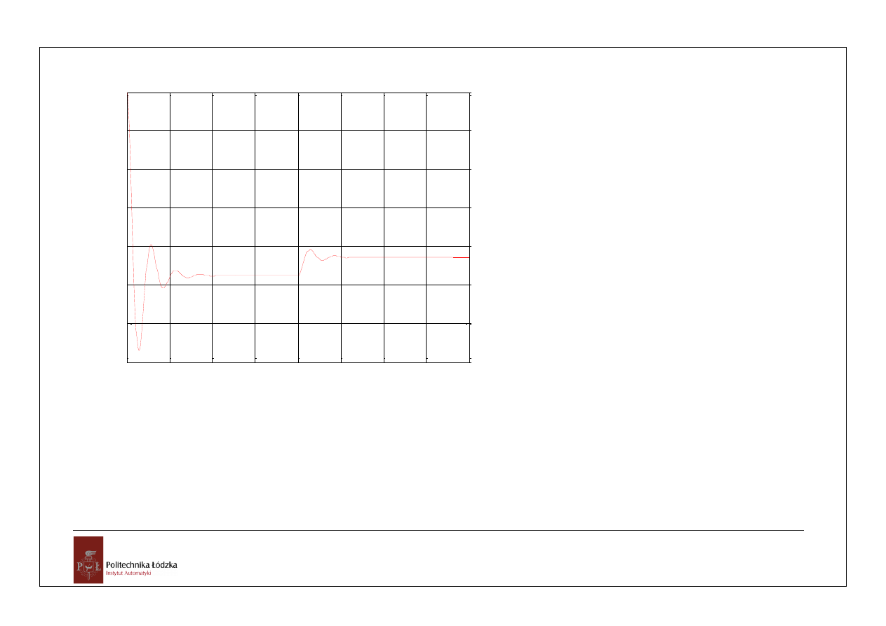
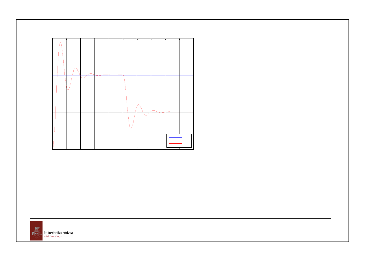
Podstawowe problemy automatyki 4
ocena pracy UAR, ćwiczenia wspomagane MATLAB-em
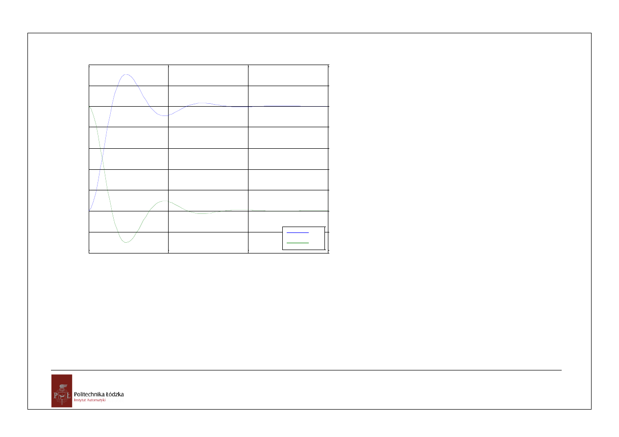
0
5
10
15
-0.4
-0.2
0
0.2
0.4
0.6
0.8
1
1.2
1.4
przebiegi w UAR
czas [s]
h
(t
),
e
(t
)
h(t)
e(t)
% Transmitancja operatorowa układu
otwartego
G0=zpk([],[0 -1],2);
% Transmitancja operatorowa układu
zamkniętego
G=feedback(G0,1);
% obliczenie odpowiedzi jednostkowej
[h,t1]=step(G,15);
% Transmitancja uchybowa
Ge=feedback(1,G0);
% obliczenie uchybu
[e,t2]=step(Ge,15);
plot(t1,h,t2,e)
grid
on
title(
'przebiegi w UAR'
)
xlabel(
'czas [s]'
)
ylabel(
'h(t),e(t)'
)
legend(
'h(t)'
,
'e(t)'
,4)

4
Podstawowe problemy automatyki 4
ocena pracy UAR, ćwiczenia wspomagane MATLAB-em
2
2
)
(
)
(
1
2
)
(
s
s
u
t
t
t
u
1
2
)
1
(
)
1
(
2
)
1
(
2
1
1
2
)
(
2
2
)
(
)
(
)
(
)
(
)
(
)
(
0
0
0
2
0
0
0
s
s
s
lim
s
s
s
lim
s
s
G
lim
s
s
sG
lim
s
u
s
sG
lim
s
se
lim
t
e
lim
e
s
s
e
s
e
s
e
s
s
t
5
Podstawowe problemy automatyki 4
ocena pracy UAR, ćwiczenia wspomagane MATLAB-em
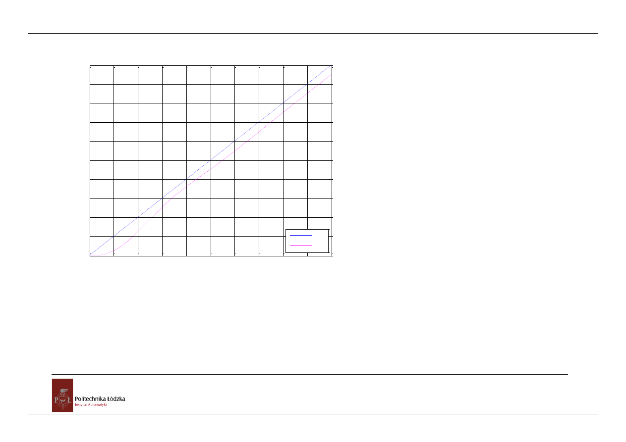
0
1
2
3
4
5
6
7
8
9
10
0
2
4
6
8
10
12
14
16
18
20
odpowiedz UAR
czas [s]
u
(t
),
y
(t
)
u(t)
y(t)
% Transmitancja operatorowa układu
otwartego
G0=zpk([],[0 -1],2);
% Transmitancja układu zamkniętego
G=feedback(G0,1)
% zdefiniowanie sygnału wejściowego
t=0:.01:10;
u=2*t;
% Odpowiedź układu na sygnał u(t)=2t
[y t1]=lsim(G,u,t)
plot(t,u,t1,y,
'm'
)
grid
title(
'odpowiedz UAR'
)
xlabel(
'czas [s]'
)
ylabel(
'u(t),y(t)'
)
legend(
'u(t)'
,
'y(t)'
,4)
6
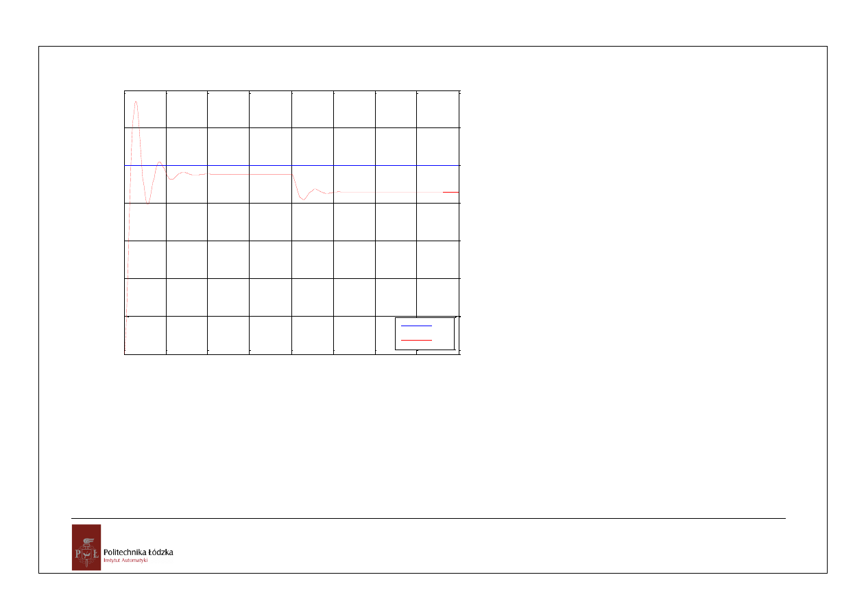
Podstawowe problemy automatyki 4
ocena pracy UAR, ćwiczenia wspomagane MATLAB-em
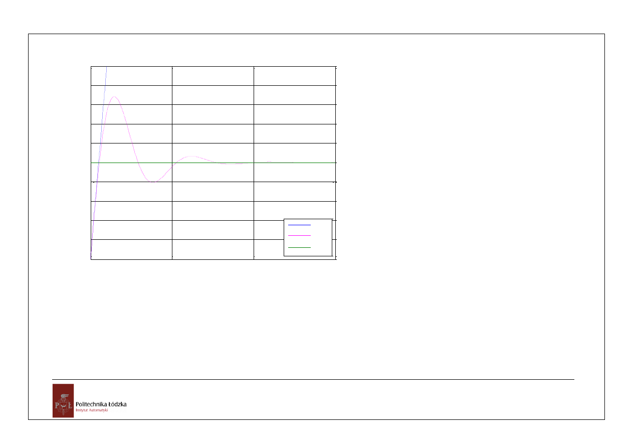
0
5
10
15
0
0.2
0.4
0.6
0.8
1
1.2
1.4
1.6
1.8
2
uchyb regulacji
czas [s]
u
(t
),
e
(t
)
u(t)
e(t)
e
u
=1
% Transmitancja operatorowa układu
otwartego
G0=zpk([],[0 -1],2);
% Transmitancja ucybowa
Ge=feedback(1,G0);
% zdefiniowanie sygnału wejściowego
t=0:.01:15;
u=2*t;
% Przebieg uchybu na sygnał u(t)=2t
[e,t1]=lsim(Ge,u,t);
plot(t(1:101),u(1:101),t1,e,
'm'
,t,t.^0)
grid
title(
'uchyb regulacji'
)
xlabel(
'czas [s]'
)
ylabel(
'u(t),e(t)'
)
legend(
'u(t)'
,
'e(t)'
,
'e_{u}=1'
,4)
7
Podstawowe problemy automatyki 4
ocena pracy UAR, ćwiczenia wspomagane MATLAB-em
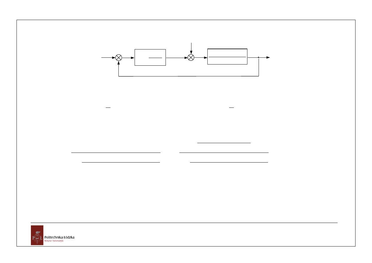
Problem 2.
W układzie jak na schemacie
10
x(s)
z(s)
1
5
,
0
04
,
0
2
2
s
s
+
_
e(s)
_
u(s)
y(s)
P
rzy zerowych warunkach początkowych podano sygnał
)
(
1
)
(
t
t
x
, a następnie
)
2
(
1
)
(
t
t
z
. Oblicz uchyb
ustalony pochodzący od wymuszenia i zakłócenia.
s
s
x
t
t
x
1
)
(
)
(
1
)
(
;
s
e
s
s
z
t
t
z
2
1
)
(
)
2
(
1
)
(
z
x
u
u
s
s
s
s
ez
s
e
s
ez
s
e
s
s
t
e
e
e
s
s
s
s
lim
s
s
lim
e
s
G
lim
s
G
lim
s
z
s
sG
lim
s
x
s
sG
lim
s
se
lim
t
e
lim
e
21
2
21
1
1
5
,
0
04
,
0
20
1
1
5
,
0
04
,
0
2
1
5
,
0
04
,
0
20
1
1
)
(
)
(
)
(
)
(
)
(
)
(
)
(
)
(
)
(
2
2
2
0
2
0
2
0
0
0
0
0
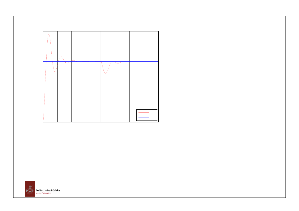
8
Podstawowe problemy automatyki 4
ocena pracy UAR, ćwiczenia wspomagane MATLAB-em
0
0.5
1
1.5
2
2.5
-0.4
-0.2
0
0.2
0.4
0.6
0.8
1
uchyb e(t) dla x(t)=1(t) przy z=0
czas [s]
e
(t
),
e
u
x
e(t)
e
u
x
% Transmitancja operatorowa obiektu
regulacji
Gor=tf([2],[0.04 0.5 1]);
% Transmitancja regulatora
Gr=tf([10],[1]);
% Transmitancja uchybowa
Ge=feedback(1,series(Gr,Gor));
% Przebieg uchybu dla x(t)=1(t), przy z=0
[h,t]=step(Ge,2.5);
plot(t,h,
'm'
,[0 2.5],[1/21 1/21],
'b'
)
axis([0 2.5 -0.4 1])
grid
title(
'uchyb e(t) dla x(t)=1(t) przy z=0'
)
legend(
'e(t)'
,
'e_{u_{x}}'
)
xlabel(
'czas [s]'
)
ylabel(
'e(t), e_{u_{x}}'
)
9
Podstawowe problemy automatyki 4
ocena pracy UAR, ćwiczenia wspomagane MATLAB-em
0
0.5
1
1.5
2
2.5
0
0.02
0.04
0.06
0.08
0.1
0.12
0.14
uchyb e(t) dla z(t)=1(t) przy x=0
czas [s]
e
(t
),
e
u
z
e(t)
e
u
z
% Transmitancja operatorowa obiektu
regulacji
Gor=tf([2],[0.04 0.5 1]);
% Transmitancja regulatora
Gr=tf([10],[1]);
% Transmitancja uchybowo - zakłóceniowa
Gez=feedback(Gor,Gr)
% Przebieg uchybu dla z(t)=1(t), przy u=0
[e,t]=step(Gez,2.5);
plot(t,e,
'm'
,[0 2.5],[2/21 2/21],
'b'
)
axis([0 2.5 0 0.14])
grid
title(
'uchyb e(t) dla z(t)=1(t) przy x=0'
)
xlabel(
'czas [s]'
)
ylabel(
'e(t), e_{u_{z}}'
)
legend(
'e(t)'
,
' e_{u_{z}}'
,4)
10
Podstawowe problemy automatyki 4
ocena pracy UAR, ćwiczenia wspomagane MATLAB-em
0
0.5
1
1.5
2
2.5
3
3.5
4
0
0.2
0.4
0.6
0.8
1
1.2
1.4
przebieg y(t) dla x(t)=1(t) i z(t)=1(t-2)
czas [s]
x
(t
),
y
(t
)
x(t)
y(t)
% Transmitancja operatorowa obiektu regulacji
Gor=tf([2],[0.04 0.5 1]);
% Transmitancja regulatora
Gr=tf([10],[1])
% Transmitancja nadążna
G=feedback(series(Gr,Gor),1)
% Transmitancja zakłóceniowa
Gz=-feedback(Gor,Gr)
% Przebieg y(t) dla u(t)=1(t)
t=0:.01:4;x=t.^0;[y,t]=lsim(G,x,t);
% Przebieg y(t) dla z(t)=1(t-2)
tz=0:.01:2;z=tz.^0;
[yz,tz]=lsim(Gz,z,tz);
a=length(t);b=length(tz);
% Przebieg y(t) dla x(t)=1(t) i z(t)=1(t-2)
yw(1:a-b,1)=y(1:a-b,1);
yw(a-b+1:a,1)=y(a-b+1:a,1)+yz(1:b,1);
plot(t,t.^0,
'b'
,t,yw,
'r'
)
grid
title(
'przebieg y(t) dla x(t)=1(t) i z(t)=1(t-
2)'
)
xlabel(
'czas [s]'
)
ylabel(
'x(t),y(t)'
)
legend(
'x(t)'
,
'y(t)'
,4)
11
Podstawowe problemy automatyki 4
ocena pracy UAR, ćwiczenia wspomagane MATLAB-em
0
0.5
1
1.5
2
2.5
3
3.5
4
-0.4
-0.2
0
0.2
0.4
0.6
0.8
1
przebieg uchybu e(t) dla x(t)=1(t) i z(t)=1(t-2)
czas [s]
e
(t
)
% Transmitancja operatorowa obiektu regulacji
Gor=tf([2],[0.04 0.5 1]);
% Transmitancja regulatora
Gr=tf([10],[1])
% Transmitancja uchybowa
Ge=feedback(1,series(Gr,Gor))
% Transmitancja uchybowo - zakłóceniowa
Gez=feedback(Gor,Gr)
% Przebieg uchybu dla u(t)=1(t)
t=0:.01:4;x=t.^0;[y,t]=lsim(Ge,x,t);
% Przebieg uchybu dla z(t)=1(t-2)
tz=0:.01:2;z=tz.^0;
[yz,tz]=lsim(Gez,z,tz);
a=length(t);b=length(tz);
% Przebieg uchybu x(t)=1(t) i z(t)=1(t-2)
yw(1:a-b,1)=y(1:a-b,1);
yw(a-b+1:a,1)=y(a-b+1:a,1)+yz(1:b,1);
plot(t,yw,
'r'
)
grid
title(
'przebieg uchybu e(t) dla x(t)=1(t) i
z(t)=1(t-2)'
)
xlabel(
'czas [s]'
)
ylabel(
'e(t)'
)
12
Podstawowe problemy automatyki 4
ocena pracy UAR, ćwiczenia wspomagane MATLAB-em
Problem 3.
W układzie jak na schemacie
s
25
,
0
1
1
5
x(s)
z(s)
1
5
,
0
04
,
0
2
2
s
s
+
_
e(s)
_
u(s)
y(s)
P
rzy zerowych warunkach początkowych podano sygnał
)
(
1
)
(
t
t
x
, a następnie
)
2
(
1
)
(
t
t
z
. Oblicz uchyb
ustalony pochodzący od wymuszenia i zakłócenia.
s
s
x
t
t
x
1
)
(
)
(
1
)
(
;
s
e
s
s
z
t
t
z
2
1
)
(
)
2
(
1
)
(
z
x
u
u
s
s
s
s
ez
s
e
s
ez
s
e
s
s
t
e
e
e
s
s
s
s
s
s
lim
s
s
s
s
lim
e
s
G
lim
s
G
lim
s
z
s
sG
lim
s
x
s
sG
lim
s
se
lim
t
e
lim
e
0
0
)
1
5
,
0
04
,
0
(
25
,
0
)
1
25
,
0
(
10
1
1
5
,
0
04
,
0
2
)
1
5
,
0
04
,
0
(
25
,
0
)
1
25
,
0
(
10
1
1
)
(
)
(
)
(
)
(
)
(
)
(
)
(
)
(
)
(
2
2
2
0
2
0
2
0
0
0
0
0
13
Podstawowe problemy automatyki 4
ocena pracy UAR, ćwiczenia wspomagane MATLAB-em
0
0.5
1
1.5
2
2.5
3
3.5
4
0
0.5
1
1.5
przebieg y(t) dla x(t)=1(t) i z(t)=1(t-2)
czas [s]
x
(t
),
y
(t
)
y(t)
x(t)
% Transmitancja operatorowa obiektu regulacji
Gor=tf([2],[0.04 0.5 1]);
% Transmitancja regulatora
Gr=tf([1.25 5],[0.25 0])
% Transmitancja nadążna
G=feedback(series(Gr,Gor),1)
% Transmitancja zakłóceniowa
Gz=-feedback(Gor,Gr)
% uchyb dla u(t)=1(t)
t=0:.01:4;x=t.^0;[y,t]=lsim(G,x,t);
% uchyb dla z(t)=1(t-2)
tz=0:.01:2;z=tz.^0;
[yz,tz]=lsim(Gz,z,tz);
a=length(t);b=length(tz);
% uchyb u(t)=1(t) i z(t)=1(t-2)
yw(1:a-b,1)=y(1:a-b,1);
yw(a-b+1:a,1)=y(a-b+1:a,1)+yz(1:b,1);
plot(t,yw,
'r'
,t,x,
'b'
)
grid
title(
'przebieg y(t) dla x(t)=1(t) i z(t)=1(t-
2)'
)
xlabel(
'czas [s]'
)
ylabel(
'x(t), y(t)'
)
legend(
'y(t)'
,
'x(t)'
,4)
14
Podstawowe problemy automatyki 4
ocena pracy UAR, ćwiczenia wspomagane MATLAB-em
0
0.5
1
1.5
2
2.5
3
3.5
4
-0.5
0
0.5
1
uchyb e(t) dla x(t)=1(t) i z(t)=1(t-2)
czas [s]
e
(t
)
% Transmitancja operatorowa obiektu regulacji
Gor=tf([2],[0.04 0.5 1]);
% Transmitancja regulatora
Gr=tf([1.25 5],[0.25 0])
% Transmitancja uchybowa
Ge=feedback(1,series(Gr,Gor))
% Transmitancja uchybowo-zakłóceniowa
Gez=feedback(Gor,Gr)
% uchyb dla u(t)=1(t)
t=0:.01:4;x=t.^0;[e,t]=lsim(Ge,x,t);
% uchyb dla z(t)=1(t-2)
tz=0:.01:2;z=tz.^0;
[ez,tz]=lsim(Gez,z,tz);
a=length(t);b=length(tz);
% uchyb u(t)=1(t) i z(t)=1(t-2)
ew(1:a-b,1)=e(1:a-b,1);
ew(a-b+1:a,1)=e(a-b+1:a,1)+ez(1:b,1);
plot(t,ew,
'r'
)
grid
title(
'uchyb e(t) dla x(t)=1(t) i z(t)=1(t-
2)'
)
xlabel(
'czas [s]'
)
ylabel(
'e(t)'
)
15
Podstawowe problemy automatyki 4
ocena pracy UAR, ćwiczenia wspomagane MATLAB-em
Problem 4.
2
x(s)
z(s)
)
1
5
,
0
04
,
0
(
2
2
s
s
s
+
_
e(s)
_
u(s)
y(s)
s
s
x
t
t
x
1
)
(
)
(
1
)
(
;
s
e
s
s
z
t
t
z
10
1
)
(
)
10
(
1
)
(
z
x
u
u
s
s
s
s
ez
s
e
s
ez
s
e
s
s
t
e
e
e
s
s
s
s
s
s
lim
s
s
s
lim
e
s
G
lim
s
G
lim
s
z
s
sG
lim
s
x
s
sG
lim
s
se
lim
t
e
lim
e
2
1
0
)
1
5
,
0
04
,
0
(
4
1
)
1
5
,
0
04
,
0
(
2
)
1
5
,
0
04
,
0
(
4
1
1
)
(
)
(
)
(
)
(
)
(
)
(
)
(
)
(
)
(
10
2
2
0
2
0
10
0
0
0
0
0
16
Podstawowe problemy automatyki 4
ocena pracy UAR, ćwiczenia wspomagane MATLAB-em
0
2
4
6
8
10
12
14
16
18
20
0
0.5
1
1.5
przebieg y(t) dla x(t)=1(t) i z(t)=1(t-10)
czas [s]
x
(t
),
y
(t
)
x(t)
y(t)
% Transmitancja operatorowa obiektu regulacji
Gor=tf([2],[0.04 0.5 1 0]);
% Transmitancja regulatora
Gr=tf([2],[1]);
% Transmitancja nadążna
G=feedback(series(Gr,Gor),1);
% Transmitancja zakłóceniowa
Gz=-feedback(Gor,Gr);
% Przebieg y(t) dla x(t)=1(t)
t=0:.01:20;x=t.^0;[y,t]=lsim(G,x,t);
% Przebieg y(t) dla z(t)=1(t-10)
tz=0:.01:10;z=tz.^0;
[yz,tz]=lsim(Gz,z,tz);
a=length(t);b=length(tz);
% Przebieg y(t) dla x(t)=1(t) i z(t)=1(t-10)
yw(1:a-b,1)=y(1:a-b,1);
yw(a-b+1:a,1)=y(a-b+1:a,1)+yz(1:b,1);
plot(t,t.^0,
'b'
,t,yw,
'r'
)
grid
title(
'przebieg y(t) dla x(t)=1(t) i
z(t)=1(t-10)'
)
xlabel(
'czas [s]'
)
ylabel(
'x(t),y(t)'
)
legend(
'x(t)'
,
'y(t)'
,4)
17
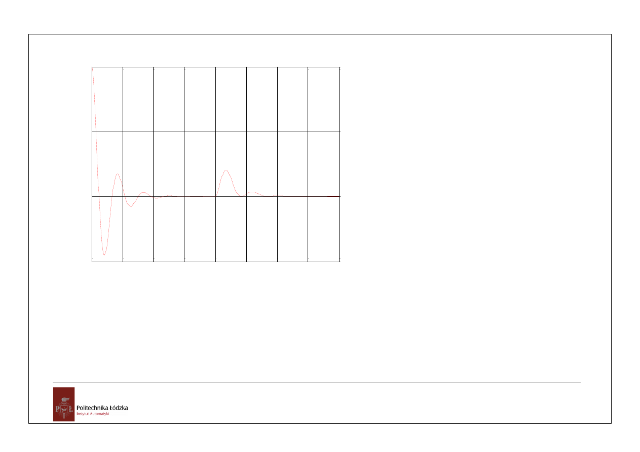
Podstawowe problemy automatyki 4
ocena pracy UAR, ćwiczenia wspomagane MATLAB-em
0
2
4
6
8
10
12
14
16
18
20
-0.5
0
0.5
1
Przebieg uchybu x(t)=1(t) i z(t)=1(t-10)
czas [s]
e
(t
)
e(t)
e
u
z
% Transmitancja operatorowa obiektu regulacji
Gor=tf([2],[0.04 0.5 1 0]);
% Transmitancja regulatora
Gr=tf([2],[1]);
% Transmitancja uchybowa
Ge=feedback(1,series(Gr,Gor));
% Transmitancja uchybowo-zakłóceniowa
Gez=feedback(Gor,Gr);
% Przebieg uchybu dla x(t)=1(t)
t=0:.01:20;x=t.^0;[e,t]=lsim(Ge,x,t);
% Przebieg uchybu dla z(t)=1(t-10)
tz=0:.01:10;z=tz.^0;
[ez,tz]=lsim(Gez,z,tz);
a=length(t);b=length(tz);
% Przebieg uchybu x(t)=1(t) i z(t)=1(t-10)
ew(1:a-b,1)=e(1:a-b,1);
ew(a-b+1:a,1)=e(a-b+1:a,1)+ez(1:b,1);
plot(t,ew,
'm'
,t,.5*t.^0,
'b'
)
grid
title(
'Przebieg uchybu x(t)=1(t) i z(t)=1(t-
10)'
)
xlabel(
'czas [s]'
)
ylabel(
'e(t)'
)
legend(
'e(t)'
,
'e_{u_{z}}'
,4)
Wyszukiwarka
Podobne podstrony:
PPA 04 2013
PPA 04 2013
PPA, wykład 7, 07 04 2017
PPA, wykład 9, 28 04 20017
Wykład 04
04 22 PAROTITE EPIDEMICA
04 Zabezpieczenia silnikówid 5252 ppt
Wyklad 04
Advanced Polyphthalamide (PPA) Metal Replacement Trends
Wyklad 04 2014 2015
04 WdK
04) Kod genetyczny i białka (wykład 4)
2009 04 08 POZ 06id 26791 ppt
2Ca 29 04 2015 WYCENA GARAŻU W KOSZTOWEJ
04 LOG M Informatyzacja log
więcej podobnych podstron