SCHOOL OF ECONOMICS

Discussion Paper 2003-05

The Random Walk Behaviour of Stock Prices:

A Comparative Study

Arusha Cooray

ISSN 1443-8593
ISBN 1 86295 130 6

The Random Walk Behaviour of Stock Prices:

A Comparative Study

Arusha Cooray

*

Abstract:

This paper tests the random walk hypothesis for the stock markets of the US, Japan, Germany,
the UK, Hong Kong and Australia using unit root tests and spectral analysis. The results based
upon the augmented Dicky Fuller (1979) and Phillips-Perron (1988) tests and spectral analysis
find that all markets exhibit a random walk. The multivariate cointegration tests based upon the
Johansen Juselius (1988, 1990) methodology indicates that all six markets share a common long
run stochastic trend. The vector error correction models suggest a short run relationship between
the US, Germany, Australia and the rest of the markets implying that these countries can gain in
the short run by diversifying their portfolios.

*

Corresponding author: Arusha Cooray, School of Economics, University of Tasmania, Private Bag 85, Hobart

Tasmania 7001, Australia. Tel: [phone]; Fax: [phone]; E-mail:

[e-mail]

1

1 Introduction

This study tests the random walk hypothesis for the stock markets of the US, Japan, Germany,

UK, Hong Kong and Australia employing stock market indices. The random-walk hypothesis

asserts that successive price changes are identically distributed independent random variables. In

an efficient market, the information contained in past prices is fully and instantaneously reflected

in current prices. Hence, the opportunity for any abnormal gain on the basis of the information

contained in historical prices is eliminated. Market efficiency would then imply that successive

price changes are independent. Most of the early studies supported the random-walk behaviour

of stock prices: Kendall (1953), Roberts (1959), Alexander (1961), Cootner (1964) and Fama

(1965), among many others.

Recent studies on stock markets reject the random walk behaviour of stock prices -

Lo, MacKinlay, Craig (1997), Taylor (200). Similarly Gallagher and Taylor (2002) show that

stock prices are not pure random walks. This study on the contrary supports the random walk

hypothesis. The random walk hypothesis is tested using the ADF (1979) and Phillips Perron

(1988) unit root tests and spectral analysis. If the unit root tests indicate that the series are

nonstationary, then they are said to follow a random walk. An alternative approach to testing for

weak form efficiency is spectral analysis which is a method of testing for oscillatory movements

in a time series. This enables identifying any cyclical or seasonal patterns in stock prices. The

random walk hypothesis claims that there are no cyclical patterns in stock prices.

2

2 Data

The data set consists of stock market indices for the US, Japan, Germany, UK, Hong Kong and

Australia. The data used is monthly and covers the period 1991.4 to 2003.2. All data series are

obtained from DATASTREAM. In order to obtain a better understanding of the data, Table 1

presents a summary of the logarithms of the first differences of the stock prices indices.

Table 1: Statistics of the First Differences of the Stock Price Indices

US

Dow

Jones

Japan

Nikkei

Germany

DAX

Britain

FTSE

100

Hong
Kong
Hang

Seng

Australia

All

Ordinaries

Maximum .10084

.15001

.41542

.10190

.26449

.078443

Minimum -.16412

-.18317

-.29327

-.21268

-.32822

-.11572

Mean .00696

-.0080

.0045

-.0025

.0062

.0046

Std Deviation

.04437

.0624

.0744

.0511

.0846

.0371

Skewness -.6656

-.06804

.39279

-.96874

-.07323

-.31270

Kurtosis-3 1.2775

-.31012

7.1779

1.7052

2.0095

-.00854

Coef of Variation

6.3691

7.7983

16.2546

19.9314

13.5928

8.0240

The data suggest that the means of the first differences for the Dow Jones, DAX, Hang Seng, and

the All Ordinaries are not far apart. For the Nikkei and FTSE 100 the means are negative. The

standard deviation of all the stock indices appear to move closely together. The first differences

of the Dow Jones, Nikkei, FTSE 100, Hang Seng and the All Ordinaries appear to be skewed to

the left while the DAX is skewed to the right. The kurtosis for the DAX is greater than 3 which

is the kurtosis of a normal distribution. For the rest of the stock indices it is less than 3. The

coefficient of variation indicates that price changes have been relatively more variable in

Germany, the UK and Hong Kong than in the US, Japan and Australia. Table 2 presents the

pairwise co-movements among the changes in stock prices. All the correlation coefficients are

positive and in the range of 0.28 and 0.71.

3

Table 2: Estimated Correlation Matrix of Variables of Stock Price Changes

Dow

Jones

Nikkei DAX

FTSE

100

Hang

Seng

All

Ords

Dow Jones

1.0000

.39675

.60792

.70960

.60394

.59694

Nikkei

.39675 1.000

.34998

.28549

.29215 .46973

DAX

.60792 .34998 1.0000

.64228

.38206 .49675

FTSE 100

.70960 .28549 .64228

1.0000

.50459 .56533

Hang Seng

.60394 .29215 .38206

.50459

1.0000 .58256

All Ords

.59694 .46973 .49675

.56533

.58256 1.0000

3 Methodology

The random walk hypothesis is tested using unit root tests and spectral analysis. Both the

augmented Dicky Fuller test and Phillips-Perron (1987, 1988) tests based upon equations (1)

and (2) are carried out to examine the univariate time series properties of the data to see if the

random walk hypothesis holds. The Augmented Dickey Fuller (ADF) unit root test is based on

the estimation of the following equation:

∆

X

t

=

β

0

+

β

1

X

t-1

+

β

2

T +

∑

=

n

i 1

β

i

∆

X

t-i

+ ε

t

(1)

where

X

t

= the time series; T = linear time trend;

ε

t

= the error term with zero mean and

constant variance. The null hypothesis of a unit root

β

1

= 0; is tested against the alternative

hypothesis,

β

1

< 0. The Z

t

statistic put forward by Phillips and Perron (1987, 1988) is a

modification of the Dickey-Fuller t statistic which allows for autocorrelation and conditional

heteroscedasticity in the error term of the Dicky-Fuller regression. This is based on the

estimation of the following:

X

t

=

α

0

+

α

1

(t-T/2) +

α

2

X

t-1

ϖ

t

(2)

4

Cointegration

The Johansen (1988) and Johansen and Juselius (1990) procedure is employed to test for a long-

run relationship between the variables. Johansen and Juselius propose a maximum likelihood

estimation approach for the estimation and evaluation of multiple cointegrated vectors. Johansen

and Juselius (1990) consider the following model:

Let X

t

be an nx1 vector of I(1) variables, with a vector autoregressive (VAR) representation of

order k,

X

t

=

Π

1

X

t-1

+ …. +

Π

k

X

t-k

+

υ

+e

t

(3)

t = 1, 2,….T

where

υ is an intercept vector and e

t

is a vector of Gaussian error terms.

In first difference form equation (3) takes the following form,

∆

X

t

=

Γ

k-1

∆

X

t-k+1

+ …. +

Π

X

t-k

+

υ

+e

t

(4)

where

Γ

i

= - ( I -

Π

1

- …

Π

i

) , for i= 1, ….. , k-1

and

Π

= - ( I -

Π

1

- ……-

Π

k

)

Π is an nxn matrix whose rank determines the number of cointegrating vectors among the

variables in X. If matrix Π is of zero rank, the variables in X

t

are integrated of order one or a

higher order, implying the absence of a cointegrating relationship between the variables in X

t

. If

Π is full rank, that is, r = n, the variables in X

t

are stationary; and if Π is of reduced rank,

5

0 < r < n,

Π can be expressed as Π = αβ' where α and β are nxr matrices, with r the number of

cointegrating vectors. Hence, although X

t

itself is not stationary, the linear combination given by

β'X is stationary.

Johansen and Juselius propose two likelihood ratio tests for the determination of the number of

cointegrated vectors. One is the maximal eigenvalue test which evaluates the null hypothesis that

there are at most r cointegrating vectors against the alternative of r + 1 cointegrating vectors. The

maximum eigenvalue statistic is given by,

λ

max

= - T ln (1 -

λ

r+1)

(5)

where

λ r+1,…,λn are the n-r smallest squared canonical correlations and T = the number of

observations.

The second test is based on the trace statistic which tests the null hypothesis of r cointegrating

vectors against the alternative of r or more cointegrating vectors. This statistic is given by

λ

trace

= -T

Σ

ln (1 -

λ

i)

(6)

In order to apply the Johansen procedure, a lag length must be selected for the VAR. A lag

length of one is selected on the basis of the Akaike Information Criterion (AIC).

1

Spectral Analysis

Spectral analysis is the study of time series in the frequency domain. The purpose of this analysis

is to determine if the stock prices exhibit any systematic cyclical variation. The sample spectrum

1

The AIC is computed as: AIC(k) = ln|

Σ

k

| + (2 p

2

k)/n , where

Σ is the residual covariance matrix; p, the number of

variables in the system; n, the number of observations and k the order of lag in the VAR.

6

is the Fourier Cosine transformation of the estimate of the autocovarience function. The Fourier

series is a representation of a function as a sum of harmonic terms such that;

f(x) =

∑

∞

=1

α

a

α

sin

α

x +1/2 a

0

+

∑

∞

=1

α

b

α

cos

α

x

or

a

0

/2 +

∑

∞

=1

α

c

α

sin (

α

x+

δ

),

where

δ = time lag and

α

= amplitude of price changes.

If

δ

is measured in radians per unit of time, sin

α

x repeats itself with period 2

π

/

α

and therefore

the number of cycles per unit or frequency is

α/

2

π.

The period

2

π

/

α

is a dimension of

t. Spectral

analysis permits the identification of any cyclical components in a data series. The angular

frequency measured in radians per unit is represented by

2

π

/

α

. Ιf p

t

, the price series,

contains a

periodic element of period k and therefore the frequency, 2

π/

k

, the spectral densities will have a

sharp spike at

α = α

k.

. If the filtered

p

t

does not contain any periodicities, the spectral densities

will be smooth.

The spectral densities of the logarithms of the prices and their first differences are estimated for

150 lags. The spectral densities are estimated as follows:

F(ϖ

j

) = 1/2π [λ

0

C

0

+ 2

λ

∑

∞

=0

K

k

C

k

cos ϖ

j

k ]

ϖ

j

=

πj/m = j = 0, 1, 2, ….m, where m = 150 lags.

The estimated autocovariance is given by,

C

k

= 1/n-k [

∑

−

=

k

n

t

1

p

t

p

t+k

– 1/n-k

∑

+

=

n

k

t

1

p

t

∑

−

=

k

n

t

1

p

t

]

7

With data,

p

t

, t = 1,…,n and the weights,

λ

k

are dependent upon

m. Microfit computes the

Bartlett, Tukey and Parzen estimates.

4 Empirical Results

Table 3 presents the time series properties of the data.

Unit Root Tests

Table 3: ADF and Phillips Unit Root Tests

Variable

Log

ADF

Levels

PP

Log First

ADF

Differences

PP

US Dow Jones

-1.53

-2.05 -13.16***

-15.04***

Japanese Nikke

-0.75

-0.86 -12.12***

-17.76***

German -1.98

-1.22

-11.09***

-13.63***

London FT

-0.29

-0.28 -10.17***

-13.71***

Hong Kong

-2.68

-3.17 -11.73***

-15.29***

Australia All-Ord

-1.59

-1.71 -13.77***

-14.58***

Note: The lag length for the ADF and Phillip-Perron regressions has been selected to ensure white noise residuals. A
fourth order autoregressive model is used for the ADF test on the basis of the AIC and ten lags on the Bartlett
window are used for the Phillip test.

Significance levels with trend: 1%, -4.07 : 5%, -3.46 : 10% -3.16; without trend: 1%, -3.51 : 5%, -2.90, 10% -2.58
(Davidson and MacKinnon 1993).

*, **, *** significant at the 10%, 5% and 1% levels respectively.

Table 3 suggests that all stock market indices are I(1) confirming the random walk hypothesis of

stock market prices and I(0) in the first differences.

8

Cointegration Tests

Table 4: Johansen-Juselius Maximum Likelihood Cointegration Test

Null Alternative

Dow Jones-Nikkei

95% critical value

mλ

Trace

mλ

Trace

r = 0

r = 1

18.86

20.75

15.87

20.18

r < = 1

r = 2

1.89

1.90

9.16

9.16

Dow Jones-DAX

r = 0

r = 1

10.47

15.71

15.87

20.18

r < = 1

r = 2

5.24

5.24

9.16

9.16

Dow Jones- FTSE 100

r = 0

r = 1

16.84

29.40

15.87

20.18

r < = 1

r = 2

12.56

12.56

9.16

9.16

Dow Jones-Hang Seng

r = 0

r = 1

9.15

16.81

15.87

20.18

r < = 1

r = 2

7.64

7.64

9.16

9.16

Dow Jones-All Ordinaries

r = 0

r = 1

15.11

18.37

15.87

20.18

r < = 1

r = 2

3.26

3.26

9.16

9.16

Nikkei-DAX

r = 0

r = 1

11.46

13.83

15.87

20.18

r < = 1

r = 2

2.36

2.36

9.16

9.16

Nikkei-FTSE 100

r = 0

r = 1

15.39

17.24

15.87

20.18

r < = 1

r = 2

1.86

1.86

9.16

9.16

Nikkei-Hang Seng

r = 0

r = 1

13.18

16.49

15.87

20.18

r < = 1

r = 2

3.30

3.30

9.16

9.16

Nikkei-All Ordinaries

r = 0

r = 1

13.76

17.10

15.87

20.18

r < = 1

r = 2

3.33

3.33

9.16

9.16

DAX-FTSE 100

r = 0

r = 1

19.78

25.31

15.87

20.18

r < = 1

r = 2

5.52

5.52

9.16

9.16

DAX-Hang Seng

r = 0

r = 1

9.94

15.16

15.87

20.18

r < =

r = 2

5.22

5.22

9.16

9.16

DAX-All Ordinaries

r = 0

r = 1

8.39

10.50

15.87

20.18

r < = 1

r = 2

2.10

2.10

9.16

9.16

9

Table 4: Continued

FTSE 100-Hang Seng Kong

r = 0

r = 1

11.43

12.66

15.87

20.18

r < = 1

r = 2

1.23

1.23

9.16

9.16

FTSE 100-All Ordinaries

r = 0

r = 1

18.86

25.11

15.87

20.18

r < = 1

r = 2

6.25

6.25

9.16

9.16

All Ordinaries-Hang Seng

r = 0

r = 1

8.74

16.03

15.87

20.18

r < = 1

r = 2

7.28

7.28

9.16

9.16

All

r = 0

r = 1

42.43

117.36

40.53

102.56

r < = 1

r = 2

30.18

74.92

34.40

75.98

r < = 2

r = 3

18.48

44.74

28.27

53.48

r < = 3

r = 4

12.89

26.25

22.04

34.87

r < = 4

r = 5

8.93

13.36

15.87

20.18

r < = 5

r = 6

4.42

4.42

9.16

9.16

The cointegration tests presented in Table 4 indicate an unique cointegrating vector for three out

of the 14 bivariate models, the Dow-Jones-FTSE 100, Dow Jones-Nikkei, DAX-FTSE 100 and

FTSE 100-All Ordinaries. There is an unique cointegrating vector for all the stock markets.

Hence the results suggest that all the markets share a common stochastic trend and departures

from this will be temporary.

Presented below are the error correction models for the markets that are cointegrated.

Bivariate Error Correction Models

Dow Jones-FTSE 100

∆DJ

t

= - 0.14

∆DJ

t-1

+ 0.10

∆FTSE

t-1

- 0.002EC

t-1

(-1.07) (0.81) (0.23)

χ

2

sc

= 16.77

χ

2

ff

= 2.44

χ

2

n

= 16.05

χ

2

hs

= 0.01

∆FTSE

t

= 0.03 ∆FTSE

t-1

+ 0.08∆DJ

t-1

- 0.05EC

t-1

(0.21) (0.56) (2.60)

χ

2

sc

= 10.61 χ

2

ff

= 1.86 χ

2

n

= 25.43 χ

2

hs

= 2.33

10

Dow Jones-Nikkei

∆DJ

t

= - 0.13

∆DJ

t-1

- 0.04

∆ΝΙΚΚΕΙ

t-1

- 0.01EC

t-1

(-1.37) (0.57) (2.5)

χ

2

sc

= 12.13

χ

2

ff

= 1.08

χ

2

n

= 27.62

χ

2

hs

= 0.15

∆NIKKEI

t

= 0.01 ∆NIKKEI

t-1

- 0.05∆DJ

t-1

- 0.05EC

t-1

(0.05) (0.37) (-2.05)

χ

2

sc

= 7.3 χ

2

ff

= 0.03 χ

2

n

= 1.2 χ

2

hs

= 0.41

DAX-FTSE 100

∆FTSE

t

= - 0.10 ∆FTSE

t-1

+ 0.06∆DAX

t-1

- 0.14EC

t-1

(0.82) (0.77) (4.14)

χ

2

sc

= 7.75 χ

2

ff

= 0.43 χ

2

n

= 35.41 χ

2

hs

= 0.11

∆DAX

t

= 0.09

∆DAX

t-1

- 0.28

∆FTSE

t-1

- 0.08EC

t-1

(0.83) (-1.53) (-3.76)

χ

2

sc

= 12.53

χ

2

ff

= 6.69

χ

2

n

= 35.41

χ

2

hs

= 4.58

FTSE 100-All Ordinaries

∆FTSE

t

= 0.02 ∆FTSE

t-1

- 0.09∆ALLORD

t-1

- 0.10EC

t-1

(0.22) (-0.67) (4.23)

χ

2

sc

= 7.75 χ

2

ff

= 0.43 χ

2

n

= 35.41 χ

2

hs

= 0.11

∆ALLORD

t

= -0.14

∆ALLORD

t-1

- 0.02

∆FTSE

t-1

- 0.07EC

t-1

(-1.29) (-0.23) (-2.96)

χ

2

sc

= 15.02

χ

2

ff

= 0.01

χ

2

n

= 2.54

χ

2

hs

= 0.01

The error correction term is of the correct sign for all the models. The error correction terms in

the Dow Jones-Nikkei, DAX-FTSE 100, FTSE 100-All Ordinaries models are significant,

suggesting a stable long run relationship between these markets. The error correction term for the

USDJ-FTSE 100 however is not statistically significant. The diagnostic tests for serial

11

correlation, functional form misspecification, and heteroscedasticity suggest that the models are

well-specified. The

χ

2

statistics for serial correlation in the models are to be compared with the

critical value of 21.03, with 12 degrees of freedom. Ramsey’s (1969) RESET test statistics for

functional form misspecification are to be compared with the 5% critical value of 3.84. It is

observed that the models are well specified. The Jarque-Bera (1980) test for the normality of

residuals indicates a non-normal distribution for the disturbance terms in all equations. This is

consistent with the distribution functions for financial assets. See Enders (2004). All equations,

support the assumption of homoscedasticity on the basis of a LM test.

Table 5: Vector Error Correction Models

Dependent
Variable

∆DJ

t-1

∆ΝΙΚΚΕΙ

t-1

∆ FTSE

t-1

∆DAX

t-1

∆HS

t-1

ALLORDS

t-1

EC

t-1

∆DJ

t

-0.51

-(3.15)

-0.20

(-0.20)

0.20

(1.50)

0.06

(0.72)

0.16

(2.41)

-0.23

(-1.26)

-0.08

(3.50)

∆FTSE

t

-0.12

(-0.60)

0.03

(0.28)

0.25

(1.50)

0.07

(0.73)

0.07

(0.92)

-0.41

(-1.90)

-0.04

(1.49)

∆NIKKEI

t

0.34

(-1.45)

0.07

(0.62)

0.42

(2.19)

0.04

(0.34)

0.08

(0.86)

-0.51

(-1.97)

-0.02

(0.69)

∆DAX

t

-0.39

(-1.43)

-0.09

(-0.71)

0.19

(0.08)

0.08

(0.61)

0.06

(0.51)

-0.17

(-0.58)

-0.16

(4.18)

∆HS

t

-0.53

(-1.66)

0.08

(0.49)

0.15

(0.58)

0.05

(0.32)

0.14

(1.09)

-0.31

(-0.86)

-0.09

(1.95)

∆ALLORD

t

-0.23

(-1.77)

-0.01

(-0.12)

0.22

(2.06)

-0.01

(-0.08)

0.11

(2.12)

-0.41

(-2.28)

-0.06

(3.41)

t statistics reported in parenthesis

Since there is an unique cointegrating vector in the six variable VAR, the short run dynamics of

the stock markets are also examined using a VECM. See Table 5. The error correction terms for

the Dow Jones, the DAX and All Ordinaries are statistically significant suggesting a short run

relationship between these markets and the rest of the stock markets.

12

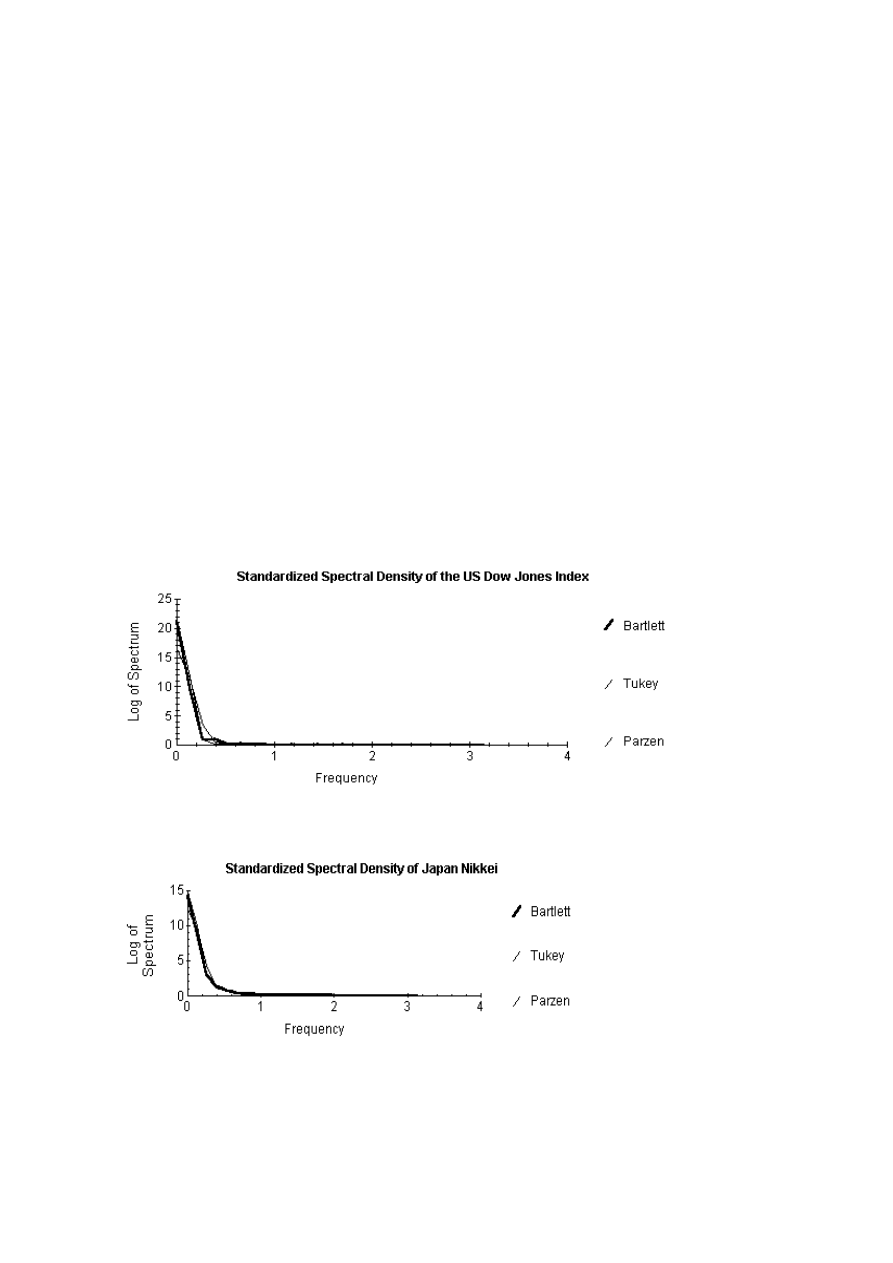
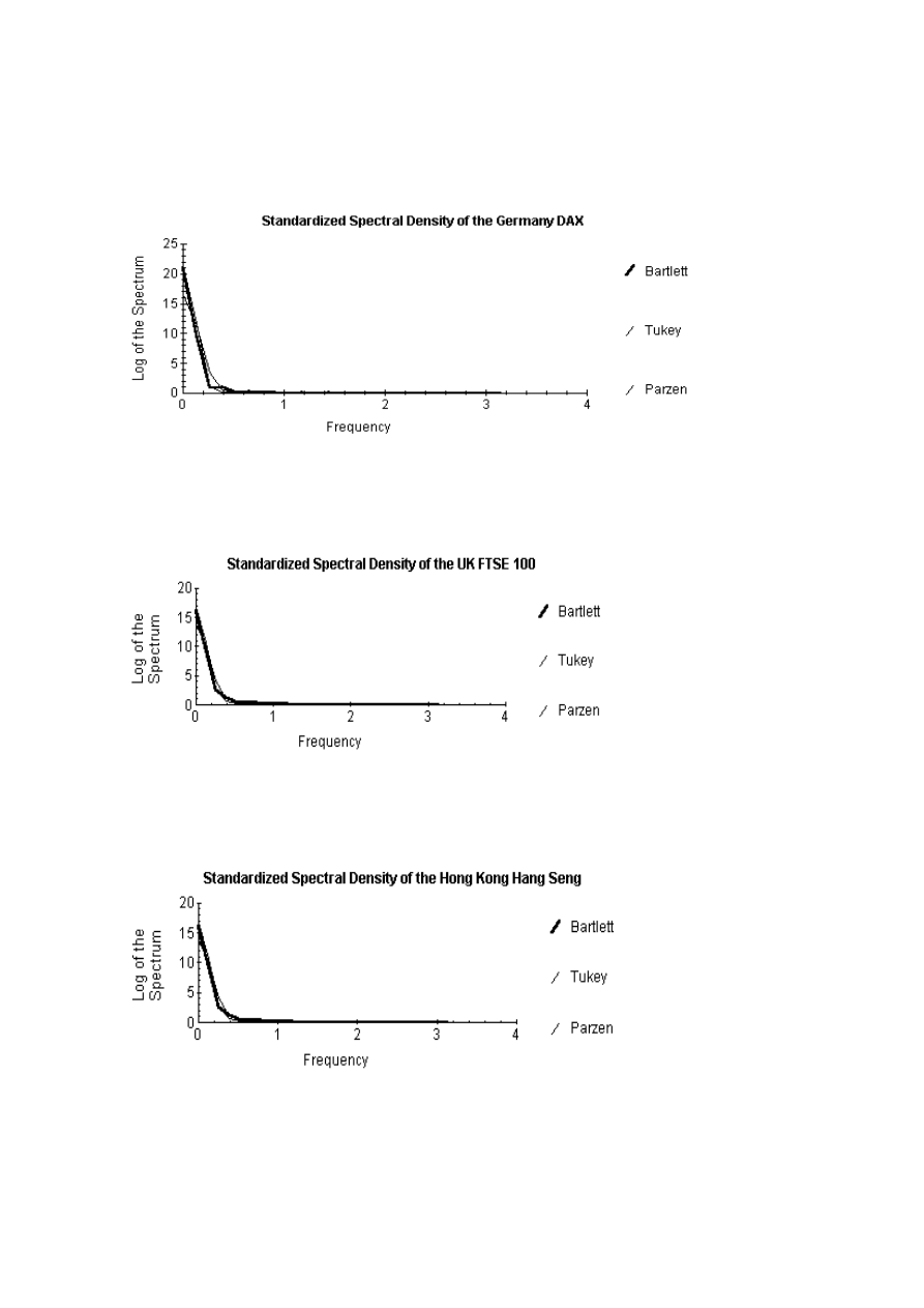
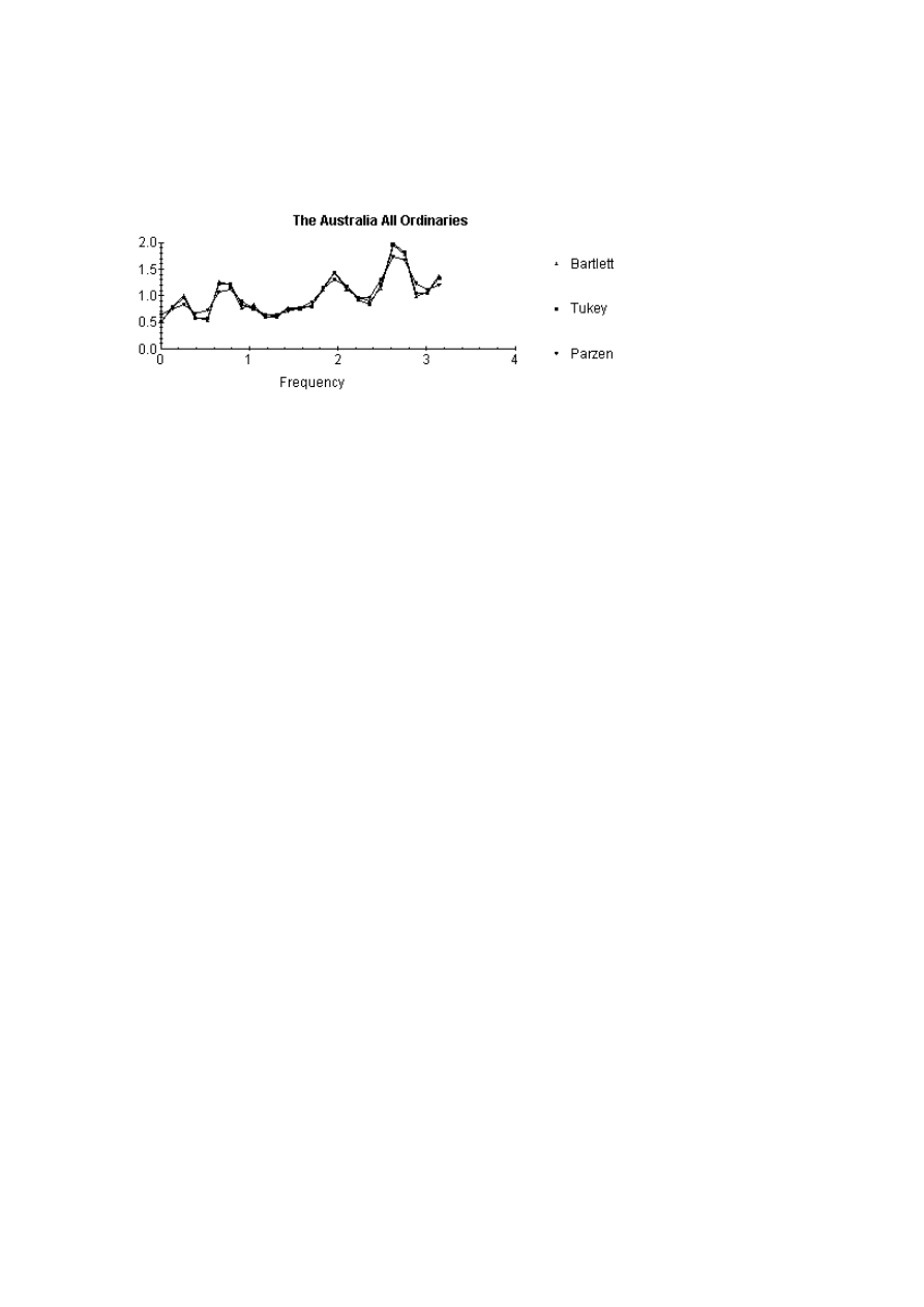
Spectral Analysis

The spectral densities are estimated for the logs of the series and the first differences of the logs

of the series. Figures 1-6 give the spectral density functions for the logs of the indices using the

Bartlett, Tukey and Parzen lag windows. These series appear to confirm the random walk

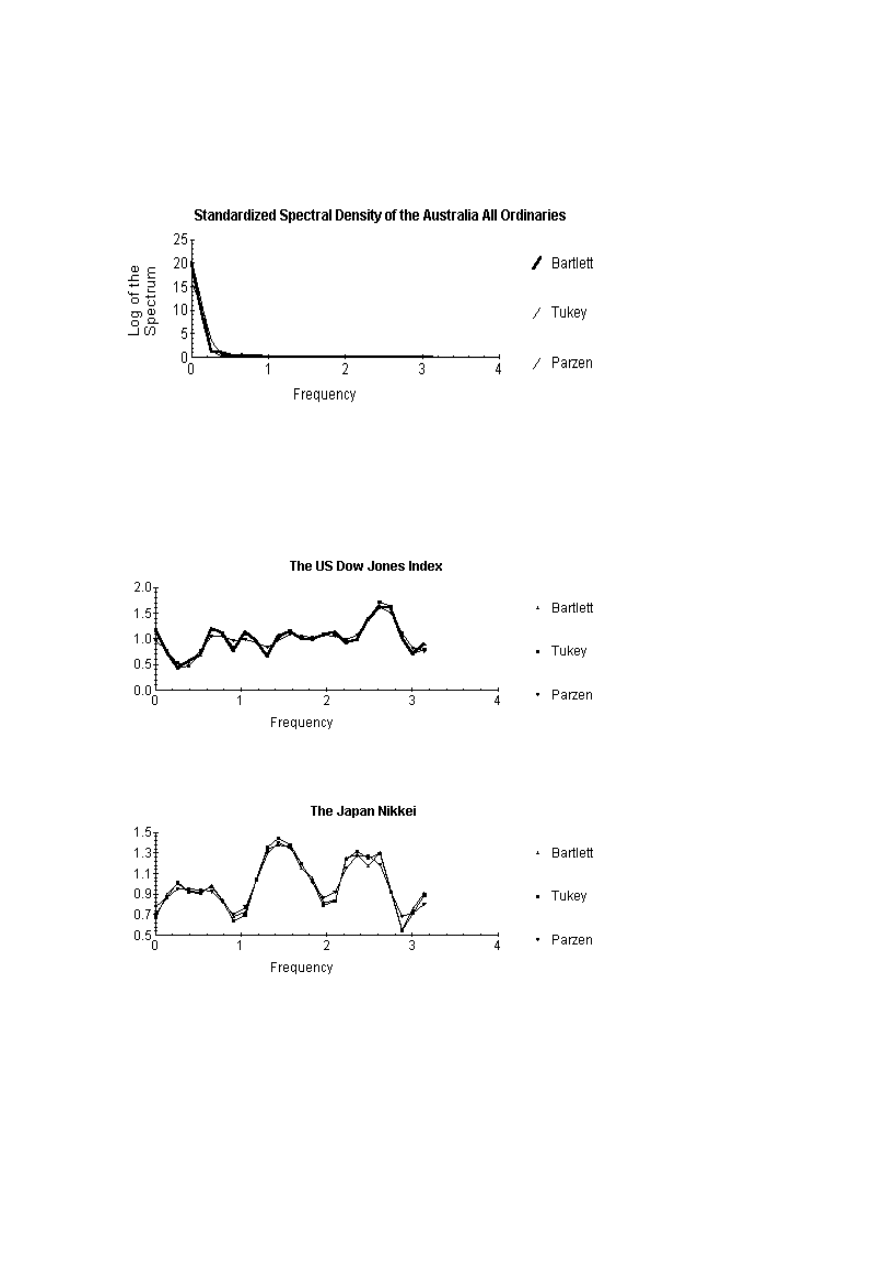
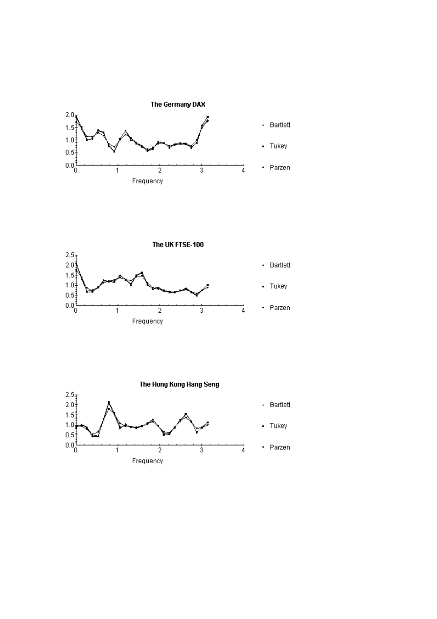
hypothesis of stock prices. Due to the non stationarity of the data, the spectral density is

controlled by the value at the zero frequency. The spectral densities are estimated for the first

differences of the series (see Figures 7-12). The first differences of the series appear to confirm

the results obtained in Table 3 that the series are I(0) in the first differences.

Figure 1

Figure 2

13

Figure 3

Figure 4

Figure 5

14

Figure 6

Standardized Spectral Density Functions of the First Differences of the Stock Price Indices

Figure 7

Figure 8

15

Figure 9

Figure 10

Figure 11

16

Figure 12

5 Conclusion

This paper has re-tested the random walk hypothesis for the stock markets of the US, Japan, the

UK, Germany, Hong Kong and Australia. The results show that contrary to recent findings that

the stock prices of these countries follow a random walk. While the Johansen-Juselius tests

suggest that all markets are cointegrated and share a long run trend, the vector error correction

models imply that the US, Germany and Australia can also stand to gain in the short term

through stock market trading.

17

References:

Alexander, S. (1961), “Price Movements in Speculative Markets: Trends or Random Walks?” in

Cootner (1964) ed.,

The Random Character of Stock Market Prices, MIT Press, MA.

Cootner, P.H. (1964), “The Random Character of Stock Market Prices,” MIT Press, MA.
Davidson, R. and MacKinnon, J.G. (1993), Estimation and Inference in Econometrics, Oxford

University Press, Oxford.

Dickey, D.A. and Fuller, W.A. (1979), “Autoregressive Time Series With a Unit Root”, Journal

of the American Statistical Association, 74, 427-431.

Enders, W. (2004), Applied Econometric Time Series, John Wiley & Sons Inc., New York.
Engle, R.F. and Granger, C.W.C. (1987), “Co-integration and Error Correction: Representation,

Estimation and Testing”, Econometrica, 55(2), 251-276.

Fama, E. (1965), “The Behaviour of Stock Market Prices”,

Journal of Business, 38,

34-105.

Gallagher, L. and Taylor, M. (2002), “Permanent and Temporary Components of Stock Prices:

Evidence from Assessing Macroeconomic Stocks”,

Southern Economic Journal, 69, 345-

362.

Jarque, C.M. and Bera, A.K. (1980), ‘Efficient Tests for Normality, Homoscedasticity and Serial

Independence of Regression Residuals”, Economics Letters, 6, 255-59.

Johansen, S. (1988), “Statistical Analysis of Cointegration Vectors”, Journal of Economic

Dynamics and Control, 12, 231-254.

Johansen, S. and Juselius, K. (1990), “Maximum Likelihood Estimation and Inference on

Cointegration – with Applications to the Demand for Money”, Oxford Bulletin of
Economics and Statistics, 52, 169-210.

Kendall, M.G. (1953), “The Analysis of Economic Time Series, Part 1: Prices,” in Cootner

(1964), ed., The Random Character of Stock Market Prices, MIT Press, MA.

Lo, A.W, MacKinlay, A.C. (1997), “Stock Market Prices Do Not Follow Random Walks”,

Market Efficiency: Stock Market Behaviour in Theory and Practice, 1, 363-389.

Phillips, P. (1987), “Time Series Regression with a Unit Root”, Econometrica, 55, 277-301.
Phillips, P. and Perron, P. (1988), “Testing for a Unit Root in Time Series Regression”,

Biometrica, 75, 335-46.

Ramsey. J.B. (1969), “Test for Specification Errors in Classical Linear Least Squares Regression

Analysis”, Journal of Royal Statistical Society, B, 350-371.

Roberts, H.V. (1959), “Stock Market ‘Patterns’ and Financial Analysis: Methodological

Suggestions”, in Cootner (1964) ed., The Random Character of Stock Market Prices, MIT
Press, MA.

Taylor, S. (2000), “Stock Index Price Dynamics in the UK and the US: New Evidence from a

Trading Rule and Statistical Analysis”, European Journal of Finance, 6, 39-69.

18

Economics Discussion Papers

2003-01

On a New Test of the Collective Household Model: Evidence from Australia, Pushkar Maitra
and Ranjan Ray

2003-02

Parity Conditions and the Efficiency of the Australian 90 and 180 Day Forward Markets,
Bruce Felmingham and SuSan Leong

2003-03

The Demographic Gift in Australia, Natalie Jackson and Bruce Felmingham

2003-04

Does Child Labour Affect School Attendance and School Performance? Multi Country
Evidence on SIMPOC Data, Ranjan Ray and Geoffrey Lancaster

2003-05

The Random Walk Behaviour of Stock Prices: A Comparative Study, Arusha Cooray

2003-06

Population Change and Australian Living Standards, Bruce Felmingham and Natalie Jackson

2003-07

Quality, Market Structure and Externalities, Hugh Sibly

2003-08

Quality, Monopoly and Efficiency: Some Refinements, Hugh Sibly

2002-01

The Impact of Price Movements on Real Welfare through the PS-QAIDS Cost of Living Index
for Australia and Canada, Paul Blacklow

2002-02

The Simple Macroeconomics of a Monopolised Labour Market, William Coleman

2002-03

How Have the Disadvantaged Fared in India? An Analysis of Poverty and Inequality in the
1990s, J V Meenakshi and Ranjan Ray

2002-04

Globalisation: A Theory of the Controversy, William Coleman

2002-05

Intertemporal Equivalence Scales: Measuring the Life-Cycle Costs of Children, Paul Blacklow

2002-06

Innovation and Investment in Capitalist Economies 1870:2000: Kaleckian Dynamics and
Evolutionary Life Cycles, Jerry Courvisanos

2002-07

An Analysis of Input-Output Interindustry Linkages in the PRC Economy, Qing Zhang and
Bruce Felmingham

2002-08

The Technical Efficiency of Australian Irrigation Schemes, Liu Gang and Bruce Felmingham

2002-09

Loss Aversion, Price and Quality, Hugh Sibly

2002-10

Expenditure and Income Inequality in Australia 1975-76 to 1998-99, Paul Blacklow

2002-11

Intra Household Resource Allocation, Consumer Preferences and Commodity Tax Reforms:
The Australian Evidence, Paul Blacklow and Ranjan Ray

Copies of the above mentioned papers and a list of previous years’ papers are available on request from the
Discussion Paper Coordinator, School of Economics, University of Tasmania, Private Bag 85, Hobart, Tasmania
7001, Australia. Alternatively they can be downloaded from our home site at

http://www.utas.edu.au/economics