Spontaneous symmetry breaking

Marcelo Mendes Disconzi

∗

Department of Mathematics, Stony Brook University

1

Introduction

The demand that the Lagrangian be gauge invariant does not allow gauge
fields to have a mass term in the Lagrangian. In other words gauge invariance
seems to imply that gauge fields are massless, because

1

m

2

A

a

A

a

is not gauge

invariant

2

.

However, in nature the carrier of exchange particles W

±

, Z-bosons have

been observed to have a mass (these are carrier particles for the weak force
between particles). On the other hand we feel very strongly that all back-
ground forces should be described by gauge fields. Spontaneous symmetry
breaking is a method by which these massive bosons can be treated under the
context of gauge theory, i.e., a way around adding the mass term m

2

A

a

A

a

to the Lagrangian which keeps gauge invariance. This is a key step in the
electroweak theory of Salam-Weinberg.

Before presenting the mechanism of symmetry breaking, we first briefly

review some facts about exchanging particles.

∗

[e-mail], URL: www.math.sunysb.edu/∼disconzi

1

The reason why this is called the mass term comes from generalizing the Klein-Gordon

equation. Recall that m

2

= E

2

− |~p|

2

from Special Relativity (with c = 1). Upon quan-

tizing: |~p|

2

7→ (−i∇)

2

and E

2

7→ H

2

, where H is the Hamiltonian (with ~ = 1). But

Schroedinger’s equation says that i∂

t

ψ = Hψ. Thus this equation in quantized form

becomes m

2

ψ = (i∂

t

)

2

ψ − (i∇)

2

ψ, i.e, ¤ψ − m

2

ψ = 0. So in the Lagrangian m

2

ψ

2

is

interpreted as the mass term.

2

To be more precise, we do know how to simply add gauge invariant mass terms (not

of the form m

2

A

a

A

a

, of course), but these turn out to be highly non-linear and in four

dimensions lead to non-renormalizable theories. The Higgs mechanism produces a mass
term which leads to a "less non-linear" (hence more treatable) and renormalizable theory.

1

2

Massive and massless particles

Let us show first that in general short range forces are massive (W

±

, Z-bosons

for the weak force) while long range forces should be massless (photon for
electromagnetism (EM) and graviton for gravity). The gluons of the strong
force are massless even though it is short range, so the idea "short range ↔
massive, long range ↔ massless" is just an approximation (but a good one,
this idea leads to the discovery of the pion which approximately describes
the strong force, see below). To proceed let us recall that the Heisenberg
uncertainty principle: ∆t∆E ≥

~
2

. This means that we need a certain amount

of time to make an accurate measurement of energy. It follows that we can
briefly violate conservation of energy without violation of quantum mechanics
(QM). For us to be able to tell the difference between two energy levels E

a

and E

b

, we must be able to measure energy to an accuracy ∆E smaller than

the difference E

a

− E

b

, i.e., ∆E ≤ E

a

− E

b

. But to measure energy to this

accuracy we must have a certain amount of time ∆t ≥

~

2(E

a

−E

b

)

, i.e., the

energy state must last for at least this period of time. So, if it does not last
at least at least

~

2(E

a

−E

b

)

, then we will not notice violations of conservation

of energy. For example, suppose we have an electron at rest. According to
Einstein E

a

= m

e

c

2

in this state. If this electron emits a photon the energy

of this new state is given by

E

b

=

m

e

c

2

q

1 −

v

2

e

c

2

= m

e

c

2

+ K

e

+ E

photon

= m

e

c

2

+ K

e

+ ~ν > E

a

where we have used that the energy of the photon equals ~ν, E

b

> E

a

implies

that energy is not conserved. Here we assume that the electron recoils when it
emits the photon so that it now has a velocity v

e

, this preserves conservation

of momentum. Even though classically this can not happen, this would not
violate QM if this photon is absorbed by another electron before the amount
of time ∆t ≥

~

2(E

a

−E

b

)

has elapsed. The absorbing electron will also recoil

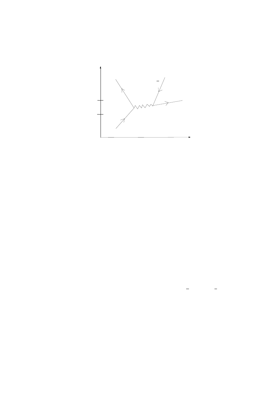
in the opposite direction to preserve momentum. The Feynman diagram
showed in figure 1.

As long as the total energy-momentum before equals the total energy-

momentum after — so, as long as the four-momentum is conserved —, this
does not violate QM, what can happen if ∆t is small. Conclusion: the

2

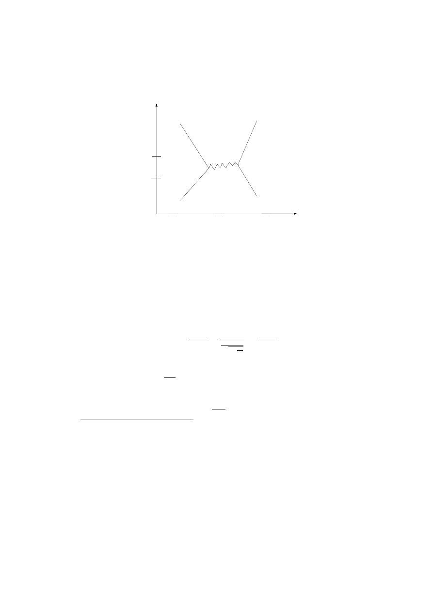
t

1

t

2

time

space

electron1

electron2

photon

Figure 1:

Electromagnetic force.

electrons have exchanged a virtual photon

3

and repelled each other. This

explains electromagnetism!

Roughly all forces should act like this

4

. Suppose we have a force mod-

erated by a massive particle, then we can get an estimate on the range of
the force. If a carrier particle of mass m is exchanged, by the uncertainty
principle the largest it can last without violate QM is

∆t ≤

~

2∆E

=

~

2mc

2

√

1−

v2

c2

≤

~

2mc

2

If we let this particle travel at nearly the speed of light, the furthest it could
travel is ∆r = c∆t ≤

~

2mc

. Thus for infinite range like gravity and EM, the

mass of their exchange particles should be zero.

The weak force has a range about 10

−18

m. Thus the mass of the weak

force exchange particle should be

~

2c∆r

≈ 10

−25

kg. Indeed, these particles

3

Of course, when carrier particles are detected by experiments they happen to be always

on-shell. Although this may sound weird, it is a typical quantum effect, similar to that
of the double slit: the electron diffracts forming and interference pattern on the wall, but
as soon as we put a detector to know by which slit it passed the interference pattern
disappears.

4

the arguments outlined here help to understand the idea short range ↔ massive, long

range ↔ massless, but they also give orders of magnitude close to the precise values (see
below).

3

have a mass of approximately 10

−25

kg

5

. Therefore this very simple reasoning

leads to a rough approximation of the masses of the carriers of the weak force.
The electroweak theory predicted the W

±

and Z bosons with the correct

masses and indeed they were discovered in 1983 at CERN. The discoverers
(of course!) won the Nobel Prize.

But even before the discovery of W

±

and Z bosons, Yukawa used ar-

guments along these lines: we know the range of the strong force between
protons and neutrons, it is about 10

−15

meters. Thus the carrier particle

should have mass around

m =

~

2c∆r

≈ 10

−27

kg

In 1925 Yukawa predicted this particle, and in 1947 the pion was discovered
with mass similar to the above value . Yukawa and Powell (the experimenter
who found it) shared the Nobel Prize for this discovery.

But this argument does not work for the strong force. Indeed, Yukawa

theory ran into a lot of difficulties in late 1950’s and early 1960’s, for exam-
ple, at very high energies the strong force could not be explained by pion
exchange. In 1964 the quark model was proposed and in this model the pion
is a bound state of a quark-antiquark pair. The strong force is now under-
stood by the exchange of gluons between quarks. Moreover, the pion is made
up of quarks and that explain why it is an approximation for carrier particles
of the strong force! The gluons have been discovered (the first direct experi-
mental evidence was in 1979) and are massless, but the strong force between
quarks acts in a very different way to all other forces: it gets stronger as
distance increases.

3

Back to spontaneous symmetry breaking

A QM system can be in various energy states given by Hψ

n

= E

n

ψ. The

state of minimum energy E

0

(not necessarily zero) is called the vacuum or

ground state. If a single vacuum state corresponds to E

0

it is said to be

non-degenerate (like for eigenvectors) and degenerate otherwise.

Suppose the system is invariant under some internal symmetry group G.

The vacuum is said to be invariant under G if it is transformed into itself
by the action of G; non-invariant otherwise. If the vacuum state and the

5

140.35 × 10

−27

kg the W boson and 160.81 × 10

−27

kg the Z boson.

4

Lagrangian are invariant under G we say the system has an exact symmetry

6

.

If the vacuum state is not invariant but the Lagrangian is, then the symmetry
is said to be spontaneously broken (or equivalently we say that the system
has a spontaneously broken symmetry). The crucial point (to be developed in
examples below) is that in order to construct a theory we must choose one of
the various vacua at hand. Although there is a symmetry relating the vacua,
we "break the symmetry" by specifying a preferred vacuum state. Finally, if
the vacuum state and the Lagrangian are not invariant then this is called an
explicit symmetry breaking.

As a very intuitive example think of a pen which is put in upright position

so carefully so that it does not fall under the influence of gravity, i.e., the
pen is in an equilibrium "state". Clearly this is very symmetric state: it is
invariant under rotations around the axis which contains the pen. However,
this equilibrium is also very unstable. Under any small perturbation the pen
will fall and reach a new equilibrium state. Now this new equilibrium state,
despite being stable, is no longer invariant under rotations, so the system
"has lost symmetry" or the symmetry is "broken".

4

Exact symmetry

We now consider several examples. The first is exact symmetry. Consider
the complex λφ

4

Lagrangian

L = ∂

a

φ∂

a

φ − m

2

|φ|

2

− λ|φ|

4

where λ is a constant called coupling constant and m is the mass of the field φ
(although coupling constants play an important role in perturbation theory,
here the reader can think of λ simply as a term which must be introduced
in order to make the last term to have the correct units). If λ 6= 0 then the
Euler-Lagrange (EL) equations are non-linear and the system is interacting

7

.

We may consider m

2

|φ|

2

+ λ|φ|

4

as a potential energy term. This Lagrangian

comes up as a simplified model for the Higgs boson, which will be discussed

6

It is worthwhile to mention that by a result of Coleman, known as Coleman’s theorem,

if the vacuum state is invariant under G so is the Lagrangian.

7

When the EL are linear the principle of superposition of solutions holds, so waves

add linearly. In other words, there is no scattering, so the theory is free; if the EL are
non-linear there will be scattering, this is why the theory is then said to be interacting.

5

later. The EL equations are

¤φ + m

2

φ + 2λφ|φ|

2

= 0

This Lagrangian is clearly invariant under the U(1) symmetry φ

0

= e

iθ

φ

(global symmetry). By calculating the stress energy-tensor we know what
the energy for this field is:

E(t) =

Z

R

3

|∂

t

φ|

2

+ ∇φ · ∇φ + m

2

|φ|

2

+ λ|φ|

4

The integrand is the energy density; usually we denote the energy density by
the same letter and call it simply "energy" (although a bit confusing, this is
a common practice, analogous to calling the Lagrangian density simply by
Lagrangian). Since all terms are positive, the minimum energy is E

0

= 0,

and the only vacuum state is φ(x) ≡ 0. Notice that this trivially satisfies
the EL equations — indeed, if we assume spatial homogeneity, which is the
case in most models, the vacuum will always satisfy EL. The vacuum is non-
degenerate since e

iθ

(0, 0) = (0, 0), showing that the vacuum is transformed

into itself under the action of the group.

5

Spontaneous breaking of global symmetry

Now consider the opposite sign for the m

2

term, i.e,

L = ∂

a

φ∂

a

φ + m

2

|φ|

2

− λ|φ|

4

The Lagrangian is still invariant under the global U(1) symmetry

8

. Now the

energy density is

E = |∂

t

φ|

2

+ ∇φ · ∇φ − m

2

|φ|

2

+ λ|φ|

4

(1)

(the total energy is the integral of the above quantity). It is clear that the
minimum of (1) is obtained when |∂

t

φ|

2

= ∇φ = 0, i.e, φ = constant and

8

Recall that a symmetry is global if its parameters are constants, e.g., φ

0

= e

iθ

φ

with θ=constant. The symmetry is local if we allow the parameters to depend on the
coordinates, e.g., φ

0

= e

iθ(x)

φ. The process of going from global to local symmetry by

allowing the parameters to depend on coordinates is referred as localizing or gauging the
symmetry and it is the starting point of gauge theories.

6

V (φ) = −m

2

|φ|

2

+λ|φ|

4

is at a minimum (this is the same thing as finding the

minimum for the function f (x) = −m

2

x

2

+ λx

4

). The critical points are at

φ = 0 and |φ|

2

=

m

2

2λ

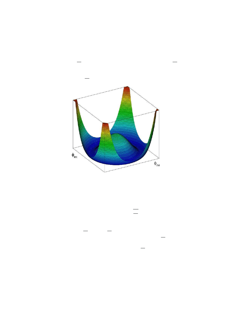
. But clearly the global minimum is at |φ|

2

=

m

2

2λ

. This

can be view from the graph of V (φ) (a "Mexican hat", see figure 2). Thus,
we get a one-parameter family of ground states, the circle in the complex
plane given by |φ|

2

=

m

2

2λ

(as before, note that this solves the EL equations).

Figure 2:

Mexican hat potential.

Therefore, we have spontaneous symmetry breaking. Indeed, These vac-

uum states are degenerate; the U(1) symmetry transformation φ

0

= e

iθ

φ

rotates these vacua along the circle. Each gets transformed into another but
never into itself (unless, of course, θ = 0).

Because the vacuum value is |φ(x)| =

q

m

2

2λ

, plugging this value into

(1) we find that the minimum energy (density) is not zero. We can shift
this expectation value in order to make it zero by changing the Lagrangian
L

0

= L − V (|φ|

2

=

m

2

2λ

) = L +

m

4

4λ

; this does not change the physics (for

example, the EL equations are the same) but now E

0

= E +

m

4

4λ

= 0.

In order to construct a theory, a definite stable vacuum — what in our

example corresponds to a point on the circle |φ|

2

=

m

2

2λ

— must be chosen. To

different vacuum states correspond different theories. This can be explained

7

because the probability of tunneling between two minima is zero. To see
this, consider the following heuristic argument from [CN]. The probability
of tunneling between two minima decreases with increasing the number of
degrees of freedom, and for an infinite number of degrees of freedom (which
is the case for a field) this probability vanishes. In fact, for a field in a
finite volume Ω the Lagrangian of a system is L

0

∼

R

d

3

xL ∼ LΩ, the

kinetic energy is ∼ |∂

t

φ|

2

Ω and the potential energy is ∼ V Ω where V =

|∇φ|

2

− m

2

|φ|

2

+ λ|φ|

2

. The problem reduces to calculating the quantum-

mechanical probability of passing a barrier of width ∼

q

m

2

2λ

and height

∼

Ωm

4

λ

by a particle of mass ∼ mΩ. This probability is proportional to

exp(−

Ωm

3

λ

) and tens to zero as Ω → ∞, i.e., transitions between two vacuum

states are not possible. Intuitively, we are saying the following: if V (φ) is
the energy density for the field then the potential energy of the system is
∼ ΩV (φ). Therefor in order to transfer the field from one ground state to
another we have to add energy proportional to ΩV (φ), what would require
infinity energy when Ω → ∞ (see [Ru] for more details).

Since any vacuum state can be transformed into another by a change of

gauge, they can all be chosen on equal footing. It is customary to choose
the one on the real axis, i.e., φ

0

=

q

m

2

2λ

, and build the theory upon this

vacuum. Small perturbations of the vacuum are excited states and are inter-
preted quantum mechanically as particles, so we consider small perturbations
around φ

0

, that is, φ(x) = φ

0

(x) + φ

1

(x) + iφ

2

(x), where φ

1

and φ

2

are real.

Plugging this into the original Lagrangian yields

L

1

(φ

1

, φ

2

) = ∂

a

(φ

0

+ φ

1

− iφ

2

)∂

a

(φ

0

+ φ

1

+ iφ

2

)

+m

2

(φ

0

+ φ

1

− iφ

2

)(φ

0

+ φ

1

+ φ

2

) − λ[(φ

0

+ φ

1

− iφ

2

)(φ

0

+ φ

1

+ iφ

2

)]

2

= ∂

a

φ

1

∂

a

φ

1

− 2m

2

φ

2

1

+ ∂

a

φ

2

∂

a

φ

2

+ L

2

where

L

2

(φ

1

, φ

2

) = −λ(φ

2

1

+ φ

2

2

)

2

− 2m

2

φ

1

(φ

2

1

+ φ

2

2

) +

m

2

2

φ

2

0

is called the interaction Lagrangian. The term

m

2

2

φ

2

0

is just a constant and

can be removed without changing the physics.

We conclude the following: spontaneous symmetry breaking of global

symmetry has lead to an equivalent theory (the Lagrangians L and L

2

are

equivalent, both describe the dynamics of the system [CN]) of a massive

8

real scalar field φ

1

and a massless real scalar field φ

2

called a Goldstone

boson (sometimes Nambu-Goldstone boson)

9

. Of course, we know that actual

symmetry in particle physics is described by local symmetry. We will see
that in that case Goldstones also appear, but only at an intermediate step;
they are not physical particles. Instead of interpreting Goldstones as physical
fields, it is more accurate to interpret them as parameterizing the orbit |φ|

2

=

m

2

2λ

. In other words, we know that in gauge theory the physical states are

the orbits (=equivalent classes of gauge related states) and a Goldstone is a
representative of such orbit.

Remark: The term m

2

|φ|

2

in the original Lagrangian is not a mass term

since it has the wrong sign and indicates imaginary mass. To find the true
mass spectrum we had to break the symmetry to get the real scalar field φ

1

with a mass term of correct sign. Thus φ

1

is the massive particle associated

to this theory and there is also a massless one, the Goldstone (see page 42 of
Chaichian/Nelipa).

6

Spontaneous symmetry breaking of local sym-
metry and Higgs mechanism

In this section we develop examples spontaneous symmetry breaking of local
symmetry.

6.1

Abelian theory

Consider EM coupled to a scalar field; the Lagrangian is

L = −

1
4

F

ab

F

ab

+ ∇

a

φ∇

a

φ + m

2

|φ|

2

− λ|φ|

4

where as usual ∇

a

φ = ∂

a

− ieA

a

φ and F

ab

= ∂

a

A

b

− ∂

b

A

a

. This Lagrangian

is invariant under the local U(1) symmetry. The total energy of the system
(which can be found with the stress-energy tensor) is

E(t) =

Z

R

3

1
2

3

X

j=1

F

2

0j

+

X

j<k

F

2

jk

+ |∇

0

φ|

2

+

3

X

j=1

|∇

j

φ|

2

− m

2

|φ|

2

+ λ|φ|

4

9

There is a surprising general fact, known as Gladstone’s theorem, which states that

spontaneous symmetry breaking of global symmetry always leads massless particles; all
such massless particles are known as Goldstones bosons.

9

(recall that the first and second sum in the integrand are the norm square
of the electric and magnetic fields E and B). The ground state must have
E = B = 0, what implies that A

a

is a closed and exact one-form, i.e., the

vector potential is what physicists call a "pure gauge": A

a

=

1
e

∂

a

α for some

α. We must also have ∇

a

φ = 0 so that ∂

a

φ − i(∂

a

α)φ = 0, what gives

φ(x) = e

iα(x)

φ

0

where as before |φ

0

|

2

=

m

2

2λ

. Therefore |φ(x)|

2

=

m

2

2λ

in order

to minimize the potential term. Note that since the energy functional is
gauge invariant, if (A

a

, φ) is a ground state then so is (A

a

+

1
e

∂

a

α, e

iα

) for

any α. We must choose one to build the theory, so we set (A

0

a

, φ

0

) = (0,

m

√

2λ

).

Since the vacuum state is not invariant under local U(1) transformations but
the Lagrangian is, we have that the system presents spontaneous symmetry
breaking.

Now we consider perturbations around the ground state: (A

a

, φ

0

+ φ

1

+

iφ

2

). Putting this into the Lagrangian produces

L

1

(φ

1

, φ

2

, A

a

) = −

1
4

F

ab

F

ab

+[∂

a

(φ

0

+ φ

1

− iφ

2

) + ieA

a

(φ

0

+ φ

1

− iφ

2

)][∂

a

(φ

0

+ φ

1

+ iφ

2

) − ieA

a

(φ

0

+ φ

1

+ iφ

2

)]

+m

2

(φ

0

+ φ

1

− iφ

2

)(φ

0

+ φ

1

+ iφ

2

) − λ[(φ

0

+ φ

1

− iφ

2

)(φ

0

+ φ

1

+ φ

2

)]

2

=

1
4

F

ab

F

ab

+

e

2

m

2

2λ

A

a

A

a

+ ∂

a

φ

1

∂

a

φ

1

− 2m

2

φ

2

1

+ ∂

a

φ

2

∂

a

φ

2

−

2me

√

2λ

A

a

∂

a

φ

2

+ L

2

(φ

1

, φ

2

, A

a

)

where L

2

is the interaction Lagrangian which consists of terms of order

greater than quadratic. Thus the vector fields has acquired a mass, and
there are now massless and massive scalar fields φ

1

, φ

2

. But now the free

part of the Lagrangian is not in canonical form — i.e., sum of quadratic
parts of Lagrangians of different fields — due to the term A

a

∂

a

φ

2

, but this

can be removed by setting B

a

= A

a

−

1

eφ

0

∂

a

φ

2

so that

L

1

(φ

1

, φ

2

, B

a

) = −

1
4

(∂

a

B

b

− ∂

b

B

a

)(∂

a

B

b

− ∂

b

B

a

) + e

2

φ

2

0

B

a

B

a

+ ∂

a

φ

1

∂

a

φ

1

−2m

2

φ

2

1

+ L

2

(φ

1

, φ

2

, B

a

)

Now we only have a massive vector field and a massive scalar field.

Therefore, we have the following conclusion: the vector field A

a

has

"eaten" a Goldstone boson φ

2

(unphysical field) and acquired a mass. This

10

is the Higgs mechanism for giving mass to gauge fields. φ

1

is called the Higgs

boson and is a physical fields which has yet to be observed. But now we
need to find how the physical fields φ

1

and B

a

transform. Under the gauge

transformation φ

0

= e

iα

φ, A

0

a

= A

a

+

1
e

∂

a

α we have, of course, that L

1

is

invariant; using φ

0

= φ

0

+ φ

0

1

+ iφ

0

2

= e

iα

(φ

0

+ φ

1

+ iφ

2

) we obtain

φ

0

1

= (φ

0

+ φ

1

) cos α − φ

2

sin α − φ

0

φ

0

2

= (φ

0

+ φ

1

) sin α + φ

2

cos α

B

0

a

= A

0

a

−

1

eφ

0

∂

a

φ

0

2

= A

a

+

1
e

∂

a

α −

1

eφ

0

∂

a

[(φ

0

+ φ

1

) sin α + α

2

cos α]

= A

a

−

1

eφ

0

(∂

a

φ

2

) cos α +

1

eφ

0

sin α∂

a

αφ

2

+

1
e

∂

a

α(1 − cos α) −

1

eφ

0

(cos α)(∂

a

α)φ

1

−

1

eφ

0

(∂

a

φ

1

) sin α

Notice that when considering infinitesimal gauge transformations — i.e. α
is small and φ

0

= φ + iαφ and A

0

a

= A

a

+

1
e

∂

a

α —, we have φ

0

1

= φ

1

and

B

0

a

= B

a

since all other terms are of order O(α). Thus in the free Lagrangian

portion of L

1

only the gauge invariant fields φ

1

,B

a

remain.

Also we should get rid of the Goldstones in L

2

, the interaction part.

This is done by choosing a gauge such that φ

0

2

= 0, what can be done by

choosing α appropriately (this is equivalent to defining a new field ψ

1

to be

a particular combination of φ

1

, φ

2

and A

a

or B

a

). But notice that after that

is no longer gauge invariant (since we are choosing a gauge [CN]), but then
only the physical fields φ

1

,B

a

remain.

Remark: The Euler-Lagrange equations for these fields are

∂

a

B

ab

+ e

2

φ

2

0

B

b

= 0

¤φ

1

+ 2m

2

φ

1

= 0

6.2

Nonabelian case

Consider the Lagrangian for a pair of self-interacting Klein-Gordon fields

L = (∂

a

φ)

H

∂

a

φ + m

2

|φ|

2

− λ|φ|

4

11

where φ = (φ

1

, φ

2

) ∈ C

2

and |φ|

2

= φ

H

φ = |φ

1

|

2

+|φ

2

|

2

. This is clearly SU (2)

invariant and we can localize this symmetry by introducing a Yang-Mills field
(i.e., a connection), so the new Lagrangian is

L = −

1
4

F

`

ab

F

`ab

+ (∇

a

φ)

H

(∇

a

φ) + m

2

|φ|

2

− λ|φ|

4

with the standard notation for Yang-Mills fields. For convenience of the
reader we recall some definitions:

A

a

(x) =

3

X

j=1

A

`

a

(x)σ

`

∈ su(2), σ

`

are generators for the algebra, i.e.:

σ

1

=

µ

0 1
1 0

¶

σ

2

=

µ

0 −i

i

0

¶

σ

3

=

µ

1

0

0 −1

¶

∇

a

φ = ∂

a

φ − igA

a

φ

F

ab

= ∂

a

A

b

− ∂

b

A

a

− i[A

a

, A

b

]

F

ab

= F

`

ab

σ

`

i.e., F = DA where D is the exterior covariant derivative; we can also write:
F

`

ab

= ∂

a

A

`

b

− ∂

b

A

`

a

+ C

km`

A

k

a

A

m

b

where the structure constants are given by

[σ

k

, σ

m

] = C

km`

σ

`

The gauge transformation is

A

0

a

= ω∂

a

ω

−1

+ ωA

a

ω

−1

φ

0

= ωφ

F

0

ab

= ωF

ab

ω

−1

where ω(x) ∈ SU(2)

The Euler-Lagrange equations are

∇

a

F

ab

= J

b

or ∂

a

F

ab

− [A

a

, F

ab

] = J

b

`

σ

`

¤φ + m

2

φ − 2λ|φ|

2

φ = 0

The current is given by

J

b

`

= i[(∇

b

φ)

H

σ

`

φ − φ

H

σ

`

∇

b

φ]

12

and the energy density by

E =

1
2

X

i

X

`

F

`

0i

F

`

0i

+

1
2

X

k<j

X

`

F

`

kj

F

`

kj

+ |∇

0

φ|

2

+

3

X

j=1

|∇

j

φ|

2

So in the ground state F

`

ij

= 0 which implies that the gauge field is a pure

gauge A

a

=

i

g

ω∂

a

ω

−1

. We must also have ∇

a

φ = 0, what gives φ(x) =

ω(x)φ

cons

(integrate by parts to see that this solves the previous equation),

where |φ

cons

|

2

=

m

2

2λ

. To choose a vacuum state to build the theory we take

A

a

= 0 and φ = (0, φ

0

) with φ

0

=

m

√

2λ

. As usual we look at perturbations

around the vacuum. These can be conveniently written as:

φ(x) = [φ

0

+ χ

0

(x)σ

0

+ iσ

`

σ

`

]

µ

0
1

¶

=

µ

χ

2

+ iχ

1

φ

0

+ χ

0

− iχ

3

¶

(σ

0

is the identity) The fields χ

1

, χ

2

, χ

3

will be Goldstones while χ

0

is the

massive Higgs field. Plugging this into the original Lagrangian yields

L(χ

0

, χ

1

, χ

2

, χ

3

, A

a

) = −

1
4

(∂

a

A

`

b

− ∂

b

A

`

a

)(∂

a

A

`b

− ∂

b

A

`a

)

+

g

2

m

2

2λ

A

`

a

A

`a

+ ∂

a

χ

0

∂

a

χ

0

− 2m

2

χ

2

0

+ ∂

a

χ

`

∂

a

χ

`

−

gm

√

2λ

A

`

a

∂

a

χ

`

+L

2

(χ

0

, χ

1

, χ

2

, χ

3

, A

a

)

where L

2

is the interaction Lagrangian consisting of terms of at least cubic

order. This appears to give three massless Goldstones χ

1

,χ

2

and χ

3

, a massive

Higgs field χ

0

and three massive gauge fields A

1

a

, A

2

a

and A

3

a

. As before,

we let the gauge fields "eat"’ the Goldstones to acquire mass by setting
B

`

a

= A

`

a

−

1

gφ

o

∂

a

χ

`

, then

L

1

= −

1
4

(∂

a

B

`

b

− ∂

b

B

`

a

)(∂

a

B

`b

− ∂

b

B

`a

) + g

2

φ

2

0

B

`

a

B

`a

+ ∂

a

χ

0

∂

a

χ

0

− 2m

2

χ

2

0

+L

2

(χ

0

, χ

1

, χ

2

, χ

3

, B

a

)

Conclusion: The Higgs mechanism for nonabelian gauge groups produces N
massive gauge fields (they acquire a mass) if the group is N dimensional and
one massive scalar (neutral, no charge) scalar field.

Remark: Again, one should choose a gauge such that χ

0

1

= χ

0

2

= χ

0

3

= 0

so that all Goldstones from L

2

vanish as well.

13

7

Electroweak theory of Glashow-Salam-Weinberg

The electroweak theory describes EM and the weak force. It illustrates (or
is based on) partial breaking of gauge symmetry and the Higgs mechanism.
The weak interaction governs β-decay in which nucleus expels an electron to
get to a lower energy configuration. This is radiation: expeltion or emission
of elementary particles from nuclei because of quantum fluctuations or in-
stability of the configuration. α-decay is when a helim nucleus is emitted as
radiation; γ-decay is when a photon is emitted as radiation.

In β-decay the weak interaction converts a neutron n

0

into a proton p

+

(which gives a radioactive isotope of the element) while emitting an electron
e

−

and an anti-neutrino ν

e

10

:

n

0

→ p

+

+ e

−

+ ν

e

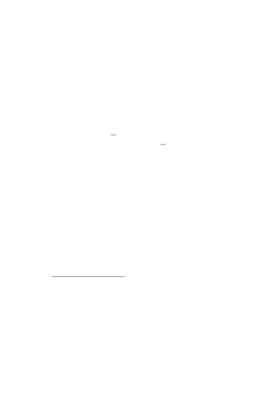
This is due to the conversion of a down quark to an up quark (in the neutron)
by emission of a W boson which subsequently decays into an electron and
anti-neutrino (see figure 3).

As primary particles for this theory one can take the electron e

−

, the µ

−

lepton, the τ

−

lepton and their neutrinos. Experimental evidence suggests

that each par particle/neutrino should have an SU(2) symmetry and thus

should be considered as a doublet

µ

ν

e

e

−

¶

,

µ

ν

µ

µ

−

¶

and

µ

ν

τ

τ

−

¶

. Since the µ

−

and τ

−

leptons are treated similarly to the electron, we restrict our attention

to the electron. Of course e

−

is represented by a 4-component Dirac field and

so is the neutrino ν

e

. The doublet ψ =

µ

ν

e

e

−

¶

is then a 8-component object

of 2 Dirac spinors. The Lagrangian is

L = ψ

H

/

∂ψ + M

2

|ψ|

2

where

/

∂ = iˆ

γ

a

∂

a

, ˆ

γ

a

=

µ

γ

a

0

0

γ

a

¶

10

Corresponding to each massive particle is an antiparticle with same mass but opposite

charge. Even electrically neutral particles such as a neutron are not identical to their
anti-particles, e.g., the neutron is made of quarks and the anti-neutron of anti-quarks.
Neutrinos are elementary particles that travel close to the speed of light, lack an electric
charge, pass through ordinary matter and have a tiny mass and are usually created from
certain radioactive decay; they interact with gravity and the weak force but not with EM
and the strong force.

14

t

1

t

2

time

space

n

0

W

+

e

−

ν

e

p

+

Figure 3:

Electromagnetic force.

This clearly has a SU(2) symmetry and a U(1) symmetry. The total group
is SU(2) × U(1) and the generators for SU (2) give the weak interaction and
for U(1) gives the EM interaction.

Experimental evidence suggests that the exchange particles for the weak

interaction have a mass so a Higgs field (massive scalar field) is needed to
import a mass to those gauge fields. We must then add to the action the
Lagrangian for the Higgs field. Since there are three generators which need to

eat three Goldstones, we need a 2 component complex scalar field

µ

φ

1

φ

2

¶

∈ C

2

to get the Higgs mechanism (three real fields will be eaten by the Goldstones
and the remaining one will be the massive Higgs). The Lagrangian is now

L = ψ

H

/

∂ψ + M

2

|ψ|

2

+ (∂

a

φ)

H

∂

a

φ + m

2

|φ|

2

− λ|φ|

4

The potential for the Higgs field and the coupling constant λ need to be
determined experimentally.

Now we need to gauge these symmetries so the Lagrangian becomes

L = ψ

H

/

∇ψ + M

2

|ψ|

2

+ (∇

a

φ)

H

∇

a

φ + m

2

|φ|

2

− λ|φ|

4

−

1
4

F

`

ab

F

`ab

−

1
4

B

ab

B

ab

where B

ab

= ∂

a

B

b

− ∂

b

B

a

is for U(1) and F

ab

= ∂

a

A

b

− ∂

b

A

a

− i[A

a

, A

b

] is for

SU(2) and ∇

a

φ = ∂

a

φ − igA

a

φ − ieB

a

φ with A

a

= A

`

a

σ

`

; also /

∇ = iγ

a

∇

a

.

15

Here g and e are coupling constants. An arbitrary gauge transformation is
given by φ

0

(x) = ω(x)e

iα

φ = e

iθ

`

σ

`

+iασ

0

φ.

We now proceed as before. A similar calculation shows that the ground

state occurs if A

a

= ω∂

a

ω

−1

, B

a

= ∂

a

α are pure gauges and ∇

a

φ = 0. This

gives φ = ωe

iα

φ

const

with |φ

const

|

2

=

m

2

2λ

. We choose as usual A

a

= B

a

= 0,

φ

const

= (0, φ

0

), φ

0

=

m

√

2λ

. The perturbations around the ground state may

be written as

φ(x) = [(φ

0

+ χ

0

)σ

0

+ iσ

`

χ

`

(x)]

µ

0
1

¶

=

=

µ

χ

2

+ iχ

1

φ

0

+ χ

0

− iχ

3

¶

Plugging into the Lagrangian yields (without the electron, i.e., we restrict to
the bosonic sector of the theory from now on):

L = −

1
4

(∂

a

A

`

b

− ∂

b

A

`

a

)(∂

a

A

`b

− ∂

b

A

`

a)∂

a

χ

0

∂

a

χ

0

− 2m

2

χ

2

0

−

1
4

(∂

a

B

b

− ∂

b

B

a

)(∂

a

B

b

− ∂

b

B

a

) +

g

2

m

2

2λ

A

`

a

A

`a

+

e

2

m

2

2λ

B

a

B

a

+∂

a

χ

`

∂

a

χ

`

−

gm

√

2λ

A

`

a

∂

a

χ

`

−

gem

2

λ

B

a

(A

3

a

−

1

gφ

0

∂

a

χ

3

) + L

1

where L

1

is the interaction Lagrangian consisting of terms of order greater

or equal to three. Letting the vector fields eat the Goldstones by ˆ

A

`

a

=

A

`

a

−

gφ

0

∂ a

χ

`

produces

L = −

1
4

(∂

a

ˆ

A

`

b

− ∂

b

ˆ

A

`

a

)(∂

a

ˆ

A

`b

− ∂

b

ˆ

A

`

a)

+

e

2

m

2

2λ

B

a

B

a

−

1
4

(∂

a

B

b

− ∂

b

B

a

)(∂

a

B

b

− ∂

b

B

a

)

+

g

2

m

2

2λ

ˆ

A

`

a

ˆ

A

`a

+ ∂

a

χ

0

∂

a

χ

0

− 2m

2

χ

2

0

−

gem

2

λ

B

a

ˆ

A

3

a

+ L

1

The new problem here is the mixed term B

a

ˆ

A

3

a

.which prevents us from de-

termining the mases of B

a

, ˆ

A

3

a

. To get rid of it we define

W

±

a

=

1

√

2

( ˆ

A

1

a

± i ˆ

A

2

a

)

Z

a

= ˆ

A

3

a

cos θ − B

a

sin θ

Y

a

= ˆ

A

3

a

sin θ + B

a

cos θ

16

where θ is a parameter to be determined. Note that the inverse transforma-
tion is

ˆ

A

1

a

=

1

√

2

( ˆ

W

+

a

+ W

−

a

)

ˆ

A

2

a

=

1

i

√

2

(W

+

a

− W

−

a

)

ˆ

A

3

a

= Z

a

cos θ + Y

a

sin θ

B

a

= Y

a

cos θ − Z

a

sin θ

Compute:

g

2

m

2

2λ

ˆ

A

3

a

ˆ

A

3a

+

e

2

m

2

2λ

B

a

B

a

−

gem

λ

B

a

ˆ

A

3a

=

m

2

λ

[(

1
2

g

2

cos

2

θ +

1
2

e

2

sin

2

θ + eg cos θ sin θ)Z

a

Z

a

+

(

1
2

g

2

sin

2

θ +

1
2

e

2

cos

2

θ − eg cos θ sin θ)Y

a

Y

a

+

+(

1
2

(g

2

− e

2

) sin 2θ − ge cos 2θ)Y

a

Z

a

]

So we choose θ such that the mixed term vanishes:

1
2

(g

2

− e

2

) sin 2θ −

ge cos 2θ = 0. The parameter θ is called mixing angle and of course de-
pends on the coupling constants. More precisely (using sin 2θ = 2 sin θ cos θ
and sin 2θ = cos

2

θ − sin

2

θ):

cos θ =

g

p

g

2

+ e

2

sin θ =

e

p

e

2

+ g

2

Notice that it follows that the coefficient in front of Y

a

Y

a

also vanishes. The

Lagrangian becomes

L = −

1
2

(∂

a

W

−

b

− ∂

b

W

−

a

)(∂

a

W

+b

− ∂

b

W

+a

) +

g

2

m

2

λ

W

−

a

W

+a

−

1
4

(∂

a

Z

b

− ∂

b

Z

a

)(∂

a

Z

b

− ∂

b

Z

a

) +

m

2

(g

2

+ e

2

)

2λ

Z

a

Z

a

−

1
4

(∂

a

Y

b

− ∂

b

Y

a

)(∂

a

Y

b

− ∂

b

Y

a

) + ∂

a

χ

0

∂

a

χ

0

− 2m

2

χ

2

0

+ L

1

Since W

−

a

= W

+

a

this corresponds to a charge massive vector field; Z

a

gives

an uncharged massive vector field and Y

a

a massless vector field; finally χ

0

17

is a massive scalar field. These are the only physical fields, .i.e., only these
combinations of the original A

`

a

and B

a

are physically meaningful. χ

0

is

of course the Higgs boson (which has yet to be detected) and naturally we
interpret Y

a

as the gauge field for the electromagnetism.

One can raise the following question: why did one vector field, Y

a

, not

acquire a mass, but the others did?

The answer is that the SU (3)×SU(2)×U(1) symmetry was only partially

broken. To see this we claim that the ground state remains invariant under
the group ˆ

U(1) with generator σ

0

+ σ

3

. Since

e

iα(σ

0

+σ

3

)

φ

cons

=

µ

e

2iα

0

0

1

¶ µ

0

φ

0

¶

=

µ

0

φ

0

¶

= φ

cons

Thus the ground state is invariant and so is the Lagrangian, hence this sym-
metry is exact and is not broken. The other three generators are broken. Note
that this subgroup ˆ

U(1) is not the standard U(1) factor of SU(2) × U(1).

This indicates that the EM potential should be a linear combination of B

a

and ˆ

A

3

a

since the group is generated by σ

0

+ σ

3

. The other three generators

which are broken and corresponding to W

±

a

and Z

a

are

1

√

2

(σ

1

±σ

2

), gσ

3

−eσ

0

or σ

3

− σ

0

.

This was an example of the Higgs mechanism with partially broken gauge

symmetry. The number of massive vector fields corresponds to the number of
broken generators. This is sometimes referred to as residual symmetry.

Under an infinitesimal ˆ

U(1) transformation φ

0

= e

iα(σ

0

+σ

3

φ with α small,

the gauge fields transform as

Z

0

a

= Z

a

χ

0

0

= χ

0

W

0±

a

= W

±

a

± iαW

±

a

Y

0

a

= Y

a

+

1
e

∂

a

α

which is another good reason for Y

a

to be identified with the EM field. Clearly

the Lagrangian is invariant under this symmetry.

Remark: As always, to get rid of the Goldstones in the interaction term

L

1

we should choose the gauge χ

0

1

= χ

0

2

= χ

0

3

= 0, so that only physical

terms remain.

18

References

[Ru]

Rubakov, V. Classical Theory of Gauge Fields. Princeton University
Press, 2002.

[CN]

Chaichian, N and Nelipa, N. F. Introduction to Gauge Field Theories.
Springer-Verlag, 1984.

[Ry]

Ryder, L. H. Quantum Field Theory. Cambridge University press,
2nd edition, 1996.

19