Techniques and

Applications for Strain

Measurements of

Skeletal Muscle

5.1

Introduction

5.2

Strain Theory

5.3

Experimental Considerations

5.4

Displacement Measurement

5.5

Conclusion

5.1 Introduction

Determination of the constitutive properties and failure tolerances has been a principal activity of solid
biomechanics for many years. Unlike engineering materials, however, the tissues and cellular structures
of the body demonstrate uniquely challenging material behavior making the measurement of constitutive
and failure properties difficult. In the face of these challenges a large experimental effort has occurred
which has resulted in an increasingly accurate determination of the tensorial quantities upon which tissue
properties and tolerances are dependent. In particular, the ability to measure stain in compliant, non-
linear, hydrated, biologic tissues has become particularly refined. Yet, the selection of the appropriate
formulation of strain, and the techniques used to measure strain vary widely. In this chapter, we present
an overview of these techniques with particular reference to the measurement of strain in muscle.

5.2 Strain Theory

A wide variety of mathematical and experimental representations have been developed to quantify the
components of strain within a deformable body. Most experimental methods quantity some component
of motion and deformation and compute the strain components of interest based on a given strain
formulation. In that regard, we present a review of deformation theory as given by Lai et al.

As a central

underlying theme, strain measurement allows a quantification of the continuous, internal deformations
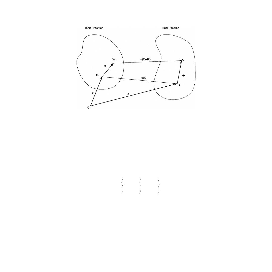
of a material which are not the result of rigid body motions. Consider the point

in the material located

a distance

from the origin (

Fig. 5.1

). As a result of a change in position,

(

), the point

is translated

to a new position

at some subsequent time. The location of the point

is described by the vector

where

(

). In that regard,

(

) represents the motion of the point

over time, where

, and

represent the components of motion in three orthogonal directions and are functions of

position on the body, (

). To describe the state of strain at the point

in the material we will

Chris Van Ee

Duke University

Barry S. Myers

Duke University

examine changes in the length between

and a closely neighboring point

. The location of

is given

. At the same subsequent time,

translates to the new location

. The new location of

given by

, and its translation is described by

(

). These quantities are related vectorially by

(

)

(5.1)

Recalling that

(

), this equation can be rewritten as

(

) –

(

) =

+ (

)

(5.2)

where

u is the displacement gradient. For Cartesian coordinates

u is given by

(5.3)

Further, we can define the deformation gradient,

, as

(5.4)

Substituting this for

in Eq. 5.2 and solving for

results in

(5.5)

where

is the identify matrix. To quantify the deformation in a small neighborhood around

compare the length of the vector

, denoted by the scalar quantity

, to the length of the vector

denoted

, resulting in the following equation:

(

)

(5.6)

FIGURE 5.1

A body undergoes a transformation described by

(

). Internal deformation is quantified by exam-

ining the mapping

and

∇ =

∂ ∂

∂













Consider the special case of rigid body motion in which

is an orthogonal matrix comprised of

orthonormal vectors such that

. Upon substitution into Eq. 5.6 results in

Subject to this condition, the length is unchanged and the deformation gradient represents a rigid body
rotation of the two points from their initial to their final positions. To define a strain tensor that is
independent of rigid body motion, it is necessary to separate out the orthogonal portion of

. Using the

polar decomposition theorem, we can write

(5.7)

where

and

are positive definite symmetric tensors and

is an orthogonal tensor representing the

rigid body motion. It can be shown that this is a unique decomposition in which

and

are known

as the right and left stretch tensors, respectively. Using Eq. 5.76, it follows that

= (

)

(

) =

(5.8)

However, because

is orthogonal,

, and Eq. 5.8 simplifies to

(5.9)

Using this formulation, several strain tensors can be defined. The right Cauchy-Green deformation tensor,

, is defined as

(5.10)

The left Cauchy-Green deformation tensor,

, is defined as

(5.11)

The Lagrangian finite strain tensor,

, is defined as

= 1/2(

–

)

(5.12)

Rewriting

in terms of the vector

results in the following expression:

= 1/2(

+ (

) + 1/2(

(

(5.13)

Expressed in tensorial notation, this gives rise to the commonly used expression

(5.14)

where m is a summed index. Each of these quantities results in a second order tensorial definition of
strain tensor. Each component of the strain tensor can be determined if the full three-dimensional
displacement field, u(u, v, w), is known. Fortunately, in many situations, it may not be necessary to use
such a generalized representation of strain. However, it should also be recognized that, even in problems
in which only the uniaxial normal strain is to be determined, the three-dimensional displacement field
may require characterization. Examination of the Lagrangian representation of strain for the character-
ization of the axial strain, E

(x, t), illustrates this phenomenon:

∂

∂
∂









 +

∂

(5.15)

In this situation, gradients of the all three deformation terms are required to characterize a single normal
strain. However, if the spatial gradients of the displacements are small, the so-called small strain problem,
the higher order terms may be neglected and the commonly used one-dimensional small strain formu-
lation

(5.16)

results. This formulation is only valid if the higher order terms remain small with respect to the first
order gradient terms. For example, a displacement gradient of

= 0.15 results in a Lagrangian strain

of 0.161. Using small strain theory, an underestimation of strain of 0.011 results, representing an error
in strain measurement of 7%.

Another commonly used convention is the stretch ratio. The stretch ratio,

λ, is defined as

(5.17)

The stretch ratio is not a tensorial component of strain. However, the stretch ratio is a convenient way
to report finite uniaxial deformations with a more obvious direct physical significance. Further, if mea-
sured in the appropriate directions, three stretch ratios can completely define other tensorial definitions
of strain, like the left Cauchy-Green strain tensor. This approach has been used together with the
assumption of incompressibility to model rubber, mesentery, muscle, and brain.

18,21,52,70,84,107,110

Ultimately, the choice of the method used to define strain will depend on the type of problem, the

constitutive formulations, and the available experimental data. Regardless of the strain formulation,
however, careful definition of the strain components measured in a given study is a requirement for the
generation of meaningful data.

5.3 Experimental Considerations

In making mechanical measurements of soft tissue, a need to reproduce the in vivo environment is
required if meaningful results are to be obtained.

14,30,44,80,116

For example, the constitutive behavior of

many biological tissues has been shown to be both temperature and hydration sensitive.

30,80

Mechanical

stabilization, or preconditioning, a process in which the tissue is cycled repeatedly at the onset of a test
battery, has also been shown to influence soft tissue behavior, and is necessary for generation of repeatable
constitutive data.

36,67,116

Soft biologic tissues are also sensitive to the loading rate and duration which can

vary from a few milliseconds during impact injury to seconds and hours in activities of daily living.

47,66,79

Several tissues, most notably skeletal muscles, undergo very large strains during physiologic loading.
Zajac reports that the tibialis anterior of the rabbit experiences a change in length between 15 and 20%
during hopping.

120

Changes in length between 10 and 50% have been reported in the lower extremity of

the cat during gait.

Using a computational model, Merrill et al. suggested that the muscles of the human

cervical spine elongate as much as 40%.

Additionally, as experimental test specimens are often removed

from their anatomic origins and insertions, specific attention to the effects of the in vitro conditions is
required. That is, the loads applied by the experimental apparatus must mimic those applied in the in
vivo environment, and the strain measurement technique must account for the effects of the nonphysi-
ologic end conditions on the measured deformation. A novel solution to this problem, which allows for
the appropriate selection of end loads, and provides estimates of in vivo loads is the measurement of
strain in vivo. Hawkins et al. measured strains of rabbit medial collateral ligament in vivo where force

x, t

( )

= ∂

∂

∂
∂









+ ∂

∂









+ ∂

∂



















1
2

x, t

( )

= ∂

∂

∂
∂

u
x

λ = ∆

measurements are impossible because of the redundant construction of the knee ligaments. The ligament
was then tested in vitro and the loads required to impose similar strains were determined and used as
estimates of the in vivo loads.

Accurate measurement of soft tissue strain is made more complex by the material heterogeneity of

biologic structures in which the soft tissues of the body often show strong regional variations. In muscle,
this includes the anatomically distinct regions of the tendons, aponeuroses, and the muscle fibers. For
example, testing of whole muscle tendon units reported in Lieber et al. resulted in average normal strains
in the mid-tendon, tendon-bone interface, and apnoneurosis of 2, 3.4, and 8%, respectively.

Variations

in the time-dependent responses of the components of muscle add a rate sensitivity to the regional
variations in strain. According to Best et al., differences in mid-muscle belly Lagrangian strains of 30%
are reported as the rate of elongation of the tendon increased from 40 to 100 cm/sec.

Strain fields also

vary from regional variations in material properties within a given muscle. As a result, even small test
specimens can have wide variations in their constitutive properties resulting from an inhomogeneous
strain field, despite having uniform test specimen geometry. Mechanical measurement in muscle is also
made more complex by the variations in area, and therefore stress, along the length of the test specimen,
as occurs commonly during whole skeletal testing.

Measurement of skeletal muscle strain is made uniquely complex by the tissue’s need to have proper

reproduction of its in vivo environment. Specifically, the mechanical properties and hence deformations
of skeletal muscle are dependent upon both a passive extracellular matrix, and a dynamic, metabolically
dependent, intracellular protein interaction. In contrast, many passive biological tissues such as bone,
ligament, tendon, and skin derive their mechanical properties exclusively from extracellular matrix
interactions. The intracellular responses depend strongly on the normal function of the cell, in addition
to the correct electrical excitation of the membrane. For these reasons, both nutrients and electrical
potentials must be supplied to the muscle during testing through either an intact neurovascular supply
or through a nutrient-rich bath using specimens of sufficiently small size to allow for the delivery of
nutrients by diffusion along. Gaining access to the tissue for deformation measurement is made increas-
ingly difficult by these additional experimental design considerations.

Considering only the passive responses, skeletal muscle still represents a complex experimental chal-

lenge. Several investigators have shown that the passive mechanical properties of skeletal muscle are a
result of mechanical load carried by both intracellular and extracellular proteins.

As a result of post-

mortem intracellular proteolysis,

102

the intracellular load carrying potential is lost, and the ability to study

cadaveric muscle is profoundly limited. Indeed, skeletal muscle experiences large changes in its mechanical
properties postmortem despite using currently accepted methods for storage of bone, ligament, tendon,
cartilage, and skin.

26,27,35,58

These changes include a decrease in stiffness of 47%,

and a decrease in strain

at failure of 44%.

Fitzgerald

26,27

reported the onset of changes in skeletal muscle mechanical properties

within the first 6 hours of death. Our own laboratory studies characterizing the mechanical properties
of skeletal muscle in the rabbit tibialis anterior support these observations (

Fig. 5.2

). The onset of rigor

can be seen as early as 6 hours postmortem. By 8 hours postmortem, stiffness increased 600% over the
live passive muscle stiffness. Following this initial stiffness increase, which peaks at 12 hours postmortem,
a gradual decrease in stiffness occurs over postmortem hours 12 to 62.5 resulting in a final muscle stiffness
which is 28% less than the live passive muscle stiffness.

Despite using methods that have been developed for storage of bone, ligament, and tendon, there are

no standardized methods to store whole muscles or cadavers through the postmortem period that
maintain the integrity of the microstructure and associated mechanical properties under the action of
postmortem enzyme activity. For this reason, investigators have developed methods to store and test
single muscle fibers.

104,105

The fibers are mechanically

78,86,87

or more often, chemically skinned

disrupting

the sarcolemma while leaving the myofibrillar structure intact. The fibers are then placed in a storage
solution where the enzyme activity is modulated, resulting in the preservation of the intracellular protein
structure. The fibers’ mechanical properties are thereby stabilized, and the tissue can be frozen for months
and tested without alterations in the mechanical properties. Further, the disruption in cell membrane

integrity allows for more direct access to the interior of the cell, allowing cell activation, relaxation, and
rigor by altering the fluid bath which surrounds the cell.

Maintaining tissue hydration for in vivo experimentation is required during testing to avoid changes

in mechanical properties due to drying.

This has been accomplished experimentally using repeated

applications of normal saline,

continuous normal saline drip,

43,58

application of a thin film of paraffin

oil,

108

immersion within a fluid bath,

covering with moist gauze,

or enclosing within a 100% humid

environment. Within muscle, an intact neurovascular supply aids in tissue hydration; however, care
should be taken to keep the surface moist. Results of hydration methods for ligament and tendon are
conflicting. Woo et al. report dehydration of tendon to cause increased stiffness and increased failure
stress.

116

Consistent with this finding is a study by Haut and Little where immersed ligaments were found

to have a decreased modulus when compared to ligaments only slightly moistened.

In contrast, a later

study by Haut and Powlinson

reported increases of 43 and 61% of tensile strength and stiffness for

immersed specimens compared to specimens moistened by a drip method of the same solution. A source
for some of these inconsistencies may be the effect of strain rate. In a study by Haut and Haut, changes
in water content of tendon had no effect on mechanical properties at a strain rate of 0.5%/s, but at a
strain rate of 50%/s, tissues with higher water content were 20% stiffer.

In an effort to better understand

the in vivo conditions and the effects of different immersion solutions, Chimich et al. measured water
content of ligament immediately after sacrifice and compared it to ligament water content after soaking
in phosphate buffered saline (PBS) and 2, 10, and 25% sucrose solutions.

Water content immediately after sacrifice was found to be 64% ± 6% while contents of PBS and the

2, 10, and 15% solutions were found to be 74, 69, 60, and 51%, respectively. Relaxation tests were
performed upon the four immersed tissues and higher water contents were associated with a greater
degree of load relaxation. However, tests on the properties of the fresh ligament were not reported. The
need to reproduce the in vivo hydration within articular cartilage is also documented. Elmore et al.
demonstrated the in vivo recoverability of articular cartilage if immersed in a balanced salt solution.

FIGURE 5.2

Structural responses of live passive skeletal muscle, and the changes in passive properties that occur

over time. The onset of rigor can be seen as early as 6 hours postmortem. By 8 hours postmortem, stiffness has
increased 600% over the live passive muscle stiffness. Following this initial increase, which peaks at 12 hours
postmortem, a gradual decrease in stiffness occurs over postmortem hours 12 to 61.5 resulting in a final muscle
stiffness which is 28% less than the live passive muscle stiffness.

contrast to tendon and ligament, the recoverability of articular cartilage was closely linked to the tonicity
of the solution. Previous experimenters testing in air had reported residual deformations after the load
had been removed and had termed this experimental artifact the “imperfect” elasticity of articular
cartilage. Appropriate selection of the hydration in the extra-specimen testing environment and careful
consideration of the importance and physiologic relevance of tissue swelling and ion movement are
therefore equally important requisites to the measurement of meaningful in vitro strains.

Temperature has also been shown to significantly affect the properties of skeletal muscle.

While the

properties of collagen have been shown to be relatively insensitive to changes in temperature ranging
from 0 to 37°C,

3,90

the properties of muscle have been shown to change over a range in temperature from

25 to 40°C.

Specifically, stiffness decreased 11 to 15% while deformation to failure was unchanged. To

standardize conditions of testing environment, a majority of investigators have chosen to use environ-
mental chambers to control both humidity and temperature.

The ability to determine the properties of soft tissue is limited because the loading conditions along

the tissue boundary are often unknown or difficult to recreate. Yet when the tissue is excised and evaluated
in vitro, recreation of these in vivo loads and boundary conditions is requisite to the generation of
meaningful constitutive data. Indeed, several investigations have shown that measured constitutive and
tolerance data depend upon the methods by which the load is applied.

10,39,116

To realize appropriate loading

conditions in vitro, investigators have developed a wide variety of gripping devices and methods.

Directly

gripping the specimen is among the most common methods used in biomechanics. Most grips compress
the tissue in a clamp with the hope of distributing the load such that the specimen neither slips in the
clamp nor suffers excessive damage in the clamp. Clamp designs are numerous and include direct
clamping by smooth or patterned metal grips, or sinusoidal shaped grips.

Capstan grips, in which the

tissue is wrapped around a cylindrical shaft and clamped, are also employed. These have the advantage
of decreasing the load on the tissue at the clamp at the expense of allowing slip in the specimen around
the capstan. However, assuming a constant coefficient of friction between capstan and grip can provide
estimates of the tissues spoolout during loading. Other approaches include the use of cyanoacrylate
adhesive, embedding the tissue in polymethacrylate, and freezing the tissue directly to the clamps.

88,95

minimize gripping effects, investigators have tested bone-tissue-bone specimens to evaluate the mechan-
ical properties of ligament, tendon, and muscle.

11,13,35

Gripping of bone results in more physiologic load

distribution in the soft tissue as the tissue’s anatomic origin and insertion are preserved. Further, the
bone is more easily gripped without risk for slip or mechanical failure at the grip site.

Variations in strain distribution near the clamp are also thought to influence results. Saint-Venant’s

principle states that end conditions whose resultant force and couple are zero will not influence the state
of stress and strain at distances that are large compared to the dimension over which the load is applied.

Experimentally, this implies that any state of stress with an equivalent resultant force and couple at the
grips will not alter the expected state of stress or strain remote from the clamps. Thus, for well-behaved
test specimens, the midsubstance stress and strain distribution will not be affected by the end conditions
and will approach the theoretical solution remote from the point of application of the load as though
an ideal load distribution had been applied. Experimentally, this requires long, slender specimens and a
path for load redistribution within the specimen that cannot always be realized with biomechanical
specimens. The significance of gripping effects was noted by Butler et al. Midsubstance tendon strains
were found to be 25 to 30% of strains near the grips or at the bone-tendon junction.

Haut reported

changes in maximum failure strain of small collagen test specimens as a function of specimen length.

Surprisingly, Haut reported maximum strains at failure of 8.1% ± 0.3%, 8.5% ± 0.6%, and 17.6% ±
1.2% for specimen gauge lengths of 100, 50, and 10 mm, respectively. Interestingly, the failure load was
insensitive to specimen length.

Increasing interest in the biomechanical behavior of cells has resulted in development of methods to

grip and measure strain on the surface of cells. Barbee et al. measured strains on the ventral cell surface
of cultured vascular smooth muscle cells.

Cell deformations were imposed by deforming the compliant

polyurethane substrate to which the dorsal surface of the cell was adherent. As in testing of larger
structures, this adhesion gripping technique has been criticized. Concerns over failure of the cell to adhere

to the membrane or cell injury as a result of membrane deformation are commonly raised. However,
Anderson et al. provide data on the strains of cultured lung, muscle, and bone cells which refute these
assertions.

They report a close agreement between cell strain and estimated membrane strain. They also

found no changes in membrane permeability, a sign of cell damage with strain, as measured by both
fluorescent and trypan blue straining techniques.

Realization of optimal clamping technique without either slip or inappropriate failure with the clamps

remains a challenge in biomechanical testing. With regard to strain measurement, the use of more
complex experimental measures of strain than simple grip-to-grip excursions can often decrease the
demands placed on clamp design and performance. That is, by measurement of full-field strain, the
effects of the end conditions on deformation can be accounted for and less constraining clamps or
enlarged grip surfaces can be employed. This is particularly relevant in failure testing in which the issue
must fail at sites remote from the clamp in order to be considered meaningful. Thus, the ease with which
the specimen can be coupled to the test apparatus often serves to define the type of strain measurement
technique which should be used.

Most measures of strain require, or are based on, a definition of the undeformed geometry or a

reference length in uniaxial problems. While often easily and uniquely defined for engineering materials
as the specimen’s zero load state, such definitions are less apparent in biologic tissues. Soft biologic tissues
are typically compliant, nonlinear, strain-stiffening materials which show a large low-load region at small
strains. As a result, small differences in the tare load (preload) used to mount the specimen can result
in profoundly different initial positions.

103

Further, creep effects under constant load can result in shifts

in a load-based initial reference length over the duration of testing. In other words, subject to a load, the
reference length changes with time. In order to manage this problem, authors have suggested fitting the
load-elongation data and extrapolating to a no-load length.

Other techniques to help define a reliable

reference length in muscle include using a gross anatomic position, a microanatomic position, or a
physiologic position. Garrett et al. established the initial length of the rabbit tibialis anterior based on
an anatomical position by measuring the muscle length when the knee and ankle were both flexed to a
joint angle of 90°.

In situ sarcomere length may also be used.

The force-length relationship of stim-

ulated skeletal muscle has also been used to define a physiologic initial position. Specifically, by electrically
twitching a muscle at various lengths the initial position of the muscle can be defined as the length at
which maximum twitch force is measured.

106

In the same context, the minimum length and maximum

length at which no force is generated in response to an electrical stimulus may also be used as a reference
length. Relationships between sarcomere length, whole muscle length, and twitch properties may allow
for comparisons of data generated using these different gauge lengths.

16,120

Measurements of the reference

state of cardiac muscle are often based on gating the position-time histories with the cardiac cycle or
cardiac electrical stimulation.

38,111,112

In either case, clear definition of a reproducible reference length is

requisite in strain measurement.

5.4 Displacement Measurement

Selection of the displacement measurement strategy is predicated on several factors including the physical
constraints imposed as a result of the need to create a physiologically appropriate testing environment
and the formulation of strain to be reported. Design considerations include the degree of intrusion
imposed by the measurement system on the tissue, the required measurement accuracy, the frequency
content of the experimental data, and the frequency response of the measurement system. Also of
importance are the need to measure surface or internal deformations and the need for real-time dis-
placements or post-test data analysis to determine displacements. Other considerations include the cost
of the system, the ease of use, the number of dimensions to be measured, and the need for average or
full-field measures of displacement. In light of the diversity of design considerations, it is of little surprise
that the techniques employed vary widely.

Like many other tissues in the body, skeletal muscle exhibits a hierarchial structural organization.

Among the most significant functional building blocks of whole skeletal muscle is the sarcomere. Indeed,

whole muscle structural properties may be derived directly from the organization of sarcomeres. Specif-
ically, force production is proportional to the numbers of sarcomeres arranged in parallel, while the
maximum tendon velocity is proportional to the number of sarcomeres in series. Sarcomere lengths range
from 1.5 to 4.0

µm and both stimulated and passive muscle responses have been shown to be functions

of the sarcomere length.

19,65,74,114

In that regard, measurement of constitutive properties as a function of

sarcomere length as opposed to strain is a common practice.

65,74

The two most common methods to

measure sarcomere length are laser diffraction and microscopy.

Microscopy affords direct observation of the tissue and has been useful in determining complex

microstructural interactions.

20,33

However, the size and proximity of the optics often preclude sarcomere

measurements during mechanical testing except for single muscle fiber preparations. In an effort to
automate sarcomere length measurements, De Clerk et al. captured microscopic images of muscle cell
striations by video.

Sarcomere lengths over a population of cardiac cells were determined by using a

Fourier transform in which the spatial frequency of the spatially periodic sarcomeres was determined.
The laser diffraction technique also makes use of the periodic structures of the sarcomeres in the muscle
fiber. Acting as a diffraction grating, a monochromatic light passing through the fibers produces a
diffraction pattern in which the distance between the first set of parallel lines is proportional to the
sarcomete length.

61,62

The laser affords the advantage of being able to measure average sarcomere lengths

through a thicker sample than compared to microscopy. As a result, dissection times are substantially
reduced using laser techniques. Laser techniques have the additional advantage of adaptability for use in
measuring in situ sarcomere length. Fleeter et al. used laser techniques to measure sarcomere length of
human forearm muscles in situ for use in tendon transfer surgeries to determine optimal muscle length
before attachment of the tendon.

Trestic and Lieber were also able to make in situ sarcomere length

measurements. Using the frog gastrocnemius muscle, in which the central tendon typically precludes
whole muscle diffraction measurements, these authors showed that diffraction measurements on partially
dissected bundles containing approximately 100 fibers compared favorably with those of the intact
muscle.

106

Lieber et al. were also able to automate the laser diffraction method to measure sarcomere

length in single muscle fiber tests. They report a frequency response of 3.8 kHz and a measurement
accuracy of 0.043

µm.

Thus, in single fiber measurement, laser diffraction techniques provide higher

frequency response but somewhat lower spatial resolution than microscopy techniques.

Analogous techniques have also been used on tendons. Sasaki and Odajima measured microstructural

deformation in tendons using X-ray diffraction.

91,92

Using a wide-angle X-ray diffraction technique,

reflections were produced corresponding to distances between neighboring amino acids along the helix
of the collagen molecule. Using small-angle X-ray diffraction, the fibrillar organization of whole collagen
molecules was measured.

Interestingly, these authors have also used microscopy techniques to measure

tendon strains, and have reported an accuracy on the order of ±0.1%.

These measurements have led

to the development of structural models based on true microstructural interactions of collagenous
tissues.

17,56,57

In contrast to microstructural measurements, tissue deformation can be measured on a macroscopic

scale using transducers which directly measure displacement. Grip-to-grip measures of displacement are
among the easiest and most commonly used. This method typically measures actuator motion for a
specimen with a grip mounted to the actuator, and another grip mounted to a fixed platen. The actuator
is usually instrumented with a linearly variable differential transformer (LVDT) which serves as a feedback
signal for the control algorithm. This signal is split, acquired digitally, and used as a measure of tissue
displacement. In that regard, the tissue motion can be measured without the use of additional instru-
mentation. While a wide variety of transducers can be used to measure displacement, the LVDT is the
most common, owing to its excellent frequency response, variable sensitivity, stability, and fatigue-
resistant design. The devices are AC transformers which detect changes in the magnetic field as a
magnetically permeable core is moved within the field. As a result, the moving core is not in direct
contact with the housing, and fatigue effects are minimized. The accuracy of the displacement measure-
ment of a typical LVDT is between 0.5 and 0.25% of full scale stroke. Full scale stroke ranges from as
little as 0.1 to 650 mm. Data can be acquired at frequencies up to 10% of the excitation frequency and

excitation frequency varies from 60 Hz to 25 kHz, although higher frequencies are attainable.

Linear

potentiometers can also measure displacement; they are considerably less expensive, approximately 10%
of the cost of an LVDT. However, they lack the sensitivity and flexibility of an LVDT and are prone to
fatigue as they operate through a contact mechanism. For strictly static measurements, dial gauges have
also been used but viscoelastic effects can confound static measurement techniques.

Dial gauges typically

provide measurement accuracies on the order of ±0.0125 mm.

While often used because of the ease of testing a whole muscle tendon unit, grip-to-grip measures are

not without limitations. The method is predicated on the use of a stiff load frame, such that test frame
deformation does not corrupt the displacement measurement. For example, Lieber et al. reported a
system compliance of 1.3

µm/g when measuring displacements of 13 mm under peak loads of 2000 g.

Another limitation with this method is the heterogeneity of the tissue between the grips. In testing whole
muscles with long tendons, the deformation of the tendon and aponeurosis can be significant, despite
subjection to smaller strains than the muscle. Trestik and Lieber report the results of an experiment in
which the gastrocnemius-Achilles tendon complex was stretched.

106

Strain within the complex varied

from 2% in the tendon up to 8% in the aponeurosis when muscle strains of 15% were observed. Clearly,
an assumption that the measured displacement could be assigned directly to the muscle would result in
substantive errors in assumed muscle strain.

Of greatest concern with this technique is the possibility of slip of the specimen within the grips,

particularly during failure testing. In general, larger measurements of deformation, and therefore strain,
are recorded when using bone-to-bone to grip-to-grip methods rather than when displacements are
measured within the tissue midsubstance.

Studies by Haut, Zernicke et al. and Butler et al. found

significant differences in the calculated modulus, failure strain, and failure strain energy density when
using grip-to-grip methods as compared to regional measures of displacement.

10,39,121

Even when slip is

minimized through the use of good gripping technique, the effects of gripping on local tissue deformation
can be significant. Zernicke et al. reported strains as great as 60% close to the grips while measured
strains remote from the grips were less than 15%. After testing gracilis, semitendinosus, fascia lata, and
patellar tendon-bone units they reported that grip-to-grip measurements of strain were 3.2 times larger
than averaged regional values through the midsection of the specimen.

121

The most common solution to the errors associated with grip-to-grip measurement in engineering

has been the use of dumbbell-shaped specimens with a midsubstance over which displacements are
measured. Clip gauges and extensometers have been commonly used to measure midsubstance displace-
ments, though they require more robust specimens than are often found in biomechanics. Clip gauges
have been developed using spring steel and other materials.

11,13

They make use of a strain gauge mounted

on an arched flexible strip formed to the desired gauge dimensions. Clips at the ends of the strip are
coupled to the tissue using glue, sutures, or clamps. Design and selection of these devices ultimately
become a trade-off between intrusion (the loads imposed on the system by the measuring device which
can alter the deformation and damage the tissue) and displacement sensitivity and frequency response.
Potentiometers and LVDTs can also be used in similar applications, although the need to maintain the
coaxial orientation of the core and housing can prove difficult.

Because of its versatility in design and very low cost, the foil strain gauge has also enjoyed popularity

as a direct contact measurement of tissue strain, although its use is limited to higher modulus materials
like bone.

Strain gauge concepts have been adapted for use with more compliant soft tissues like tendon

and ligament. For example, liquid metal strain gauges make use of mercury-filled silastic tubes that are
sutured directly to the surface of the tissue. Described in detail by Brown et al. and Meghan et al., these
devices operate through the same mechanism as the foil gauge.

9,68

As the tube’s length is changed, the

cross section is altered and the resistance changes. Meglan et al. used this gauge to measure anterior
cruciate ligament strain.

Van Weeren et al. measured the in vivo strains of the peroneous tertius tendon

of a horse.

109

Brown et al. measured the dynamic performance of these gauges and their applicability to

measurements of soft tissue strain.

The gauges were found to be linear up to 40% change in length. In

addition, gauges exhibited frequency independent response up to 50 Hz for a cyclic 20% change in length.
Stiffness of the gauge was found to be 0.024 N/mm, which is approximately 4% that of tendon. However,

the shelf life of the gauges is limited to about 3 months due to the oxidation of the mercury through the
silastic tubing.

Arms et al. used a Hall effect sensor to estimate strains in the medial collateral ligament.

A semicon-

ductor device measured the proximity of a permanent magnet attached to the tissue. Cholewicki et al.
also employed a Hall effect device to measure motion between the facet surfaces of the intervertebral
joint.

The device’s range of motion was 4 to 12 mm with a reported accuracy of 0.025 mm. Frequency

response of the sensor was reported to be 20 kHz; however, mass effects associated with the guide track,
sensor, and magnet will likely limit frequency performance to a value considerably below the sensor
response. Additionally, the calibration of this device was nonlinear, making its use somewhat more
difficult. While the cost of a Hall effect sensor is typically less than a dollar, the mounts must be designed
and assembled by the investigator. Commercially available sensors are available; the cost is approximately
$900.

Villarrel et al. and Omens et al. describe the use of three piezoelectric crystals to determine planar

displacements of the left ventricle of the heart. Each crystal both receives and transmits signals to the
other two crystals resulting in measures of length based on assumptions regarding transmission velocity
in the media. Frequency response of the system was 375 Hz. Accuracy of the system was not calculated,
but results were similar to those derived from using biplane coneradiography.

82,111

George and Bogen report the design, construction, and use of a novel biaxial fiberoptic strain gauge

system.

The system employs 0.76 mm diameter fiber optic cables which are inserted transversely through

the substance of the tissue and direct light onto a large silicon photo diode which tracks the point at
which the light contacts the diode array. The system is synchronized so that as each fiber is illuminated
in order, the diode output is sent to a multiplexer resulting in a system frequency response of approxi-
mately 3 kHz. The authors noted that hardware cost was approximately $1000. That figure did not include
the circuit design, construction, testing, or calibration. The authors used this prototype device to measure
tissue strains as large as 40% during a biaxial test of a flat section of the ovine right ventricle. As the
fibers are transversely mounted through the section of tissue, their intrusion on the deformation was
thought to be minimal. The accuracy and calibration of this method are not reported. Further, the errors
due to optic fiber rotation or distortion across the cross section of the tissue that would result from a
nonuniform strain field were not discussed.

Because direct contact methods using transducers are invasive, and rarely provide full-field measures

of strain, noncontact methods have become increasingly more popular. These methods typically track
the position of tissue markers over time to determine displacements at discrete points of the tissue and
are commonly used to determine the full-field strain variation across the tissue. Obtaining tissue marker
contrast and quantifying marker position are achieved using a wide variety of tools and techniques
including clinical imaging systems and optical methods. Clinical imaging systems have the advantage of
being able to capture images of the tissue when the region of interest cannot be directly visualized using
optical methods.

Biplanar cineradiography is among the most common and oldest techniques, and has been used in a

variety of applications including determining the deformations in a three-dimensional space of the
beating canine heart in vivo.

38,112

A number of studies have investigated the methods used for deriving

the three-dimensional space from the planar images and the results of a parametric analysis of the errors
associated with biplanar cineradiography have been reported.

1,45,63,72,98,115

Hashima et al. used this method

to track the positions of an array of 25 lead beads (1.0 mm in diameter) sewn to the epicardium of the
left ventricle in an array approximately 5 to 10 mm apart.

Frames were captured at a rate of 120 Hz

but other studies report using frequencies up to 3000 Hz.

To calibrate the system, several 1.0 cm long

radiopaque rods were placed within the field and imaged. In a similar study, Waldman et al. found the
error in the reconstruction of the three-dimensional displacements using biplanar cineradiography to be
0.3 mm and was limited primarily by digitization errors.

112

Pin cushion distortion (warping along the

edges of the image) and the cone effect (magnification dependent on distances from the focal plane)
were relatively small compared to the digitizing errors (0.05 and 0.1 mm, respectively). In a later study
examining errors associated with this method, Waldman and McCulloch reported that marker positions

could be located in three-dimensional space with a standard deviation of 2.5% of the full-field of view
using biplane cineradiography.

113

The recent use of magnetic resonance tagged images has eliminated the need for the invasive implantation

of radiopaque markers into the tissue associated with biplanar cineradiography. The technique is based on
locally perturbing the magnetization of the myocardium with selective radio-frequency saturation, resulting
in multiple, thin tag planes. The imaging plane is orthogonal to the tag planes and the intersections of these
planes result in dark stripes withich deform with the tissue. The intersections are tracked, resulting in a
spatial history of the tissue deformation. Young et al. reported using this method to track the deformations
of the human heart. A total of 3100 points were tracked with an RMS error of half a pixel or 0.47 mm.

119

Studies by other investigators reported similar point location accuracy of approximately 0.3 mm.

53,81

obvious advantage of the magnetic resonance tagging methods is the noninvasive ability to track the motion
of an entire tissue volume including the tissue substance and the tissue surface in vivo. Current techniques,
however, remain limited by the frequency and duration over which these images may be obtained and the
number of institutions equipped to perform these measurements.

Optical methods have been widely used and include still photography,

100

video,

43,36,85,121

and CCD (charge

coupled device) cameras.

8,108

These systems track optical markers or tissue landmarks on the surface of the

tissue to determine displacements. A great number of different optical markers have been used. Markers
vary in size, shape, color, and material. Selection of an appropriate marker aids in tracking, improving
accuracy, and minimizing the effect of the marker on strain profile. Accuracy of each of these techniques
seems most tightly coupled to reliably determining an exact marker location during digitization.

100

Improving marker contrast to gain accuracy and ease of marker tracking has been studied extensively.

Non-reflective markers can be made by blackening a surface with sulfide, ink, or paint. Fluorescent
markers have also been used.

7,99

Smutz et al. used fluorescent markers illuminated by an ultraviolet light

source in an otherwise dark room. Others have relied on tissue-mounted LEDs. These methods have the
advantage of allowing band pass filtering at the excitation frequency to improve contrast between the
markers and the background.

46,108

In addition to marker contrast, the attachment of the marker to the tissue requires careful consider-

ation. Hoffman and Grigg used stopcock grease or mineral oil to attach 600

µm disks to the posterior

joint capsule of the cat knee.

Other methods to attach markers are the use of histoacryl glue,

85,108

cyanoacrylate glue,

100

and small sutures.

12,38

The attachment of external markers to the tissue is not

without consequences. Barbee et al. validated their method of bead attachment to single smooth muscle
cells by microscopically examining the substructure with and without the beads attached to insure that
the cell did not reorganize with the addition of the 10

µm diameter microspheres.

Investigators have

also stained the tissue of interest directly with paints or ink to avoid the problems of external marker
attachment. Elastin stain,

106

Verhoeff ’s stain,

and India ink have all been used.

8,10,121

While decreasing

intrusion, stains typically create irregular marks with varying signal intensities whose locations may be
more difficult to determine.

A majority of these methods involve placing the marker on the surface of the tissue, thus only providing

data about the displacements at the surface. In an effort to measure the deformations within the substance
of articular cartilage, Schinagl et al. used fluorescently stained cell nuclei as markers.

Nuclei at different

depths were then tracked using transmitted and epifluorescence microscopy.

In order to track the marker displacement, an image capture technique needs to be implemented. For

static testing, a low method to track marker displacement is photography.

100

The shutter time or acqui-

sition time of a single frame must be quick enough to avoid blurring of the markers in the image. Typical
video systems have a frequency response of 30 Hz, but split frame video at 60 Hz is also common.

118

avoid blurring of moving markers during the long exposure times of conventional video. Prinzen et al.
incorporated the use of a xenon strobe which was triggered by a video frame pulse.

Hoffman and Grigg

described a method using a high-sensitivity television camera, a trinocular microscope, and a video image
frame grabber to store the digitized image on a microcomputer for post-processing.

Other investigators

have recorded their images using CCD cameras that allow image acquisition rates up to and greater than
10 kHz.

8,108

Microscopes can be used in conjunction with video or CCD cameras to track the positions

of small particles.

7,93

Polaroid filters have also been used to eliminate unwanted glare associated with

moist tissues.

For three-dimensional measurements of displacement, two or more image views are obtained and

reconstructed through the use of direct linear transformation methods.

6,1,50,51,64,97

Sirkis and Lim described

the equations used for a direct linear transform assuming a pin-hole camera, and investigated the role
of possible errors in the process.

Luo et al. examined the effects of changing the angle between the two

cameras used to quantify the three-dimensional space.

A lower limit of the pan angle was found to be

20 degrees. No improvement in accuracy was noted as pan angles increased to 40 degrees and testing at
larger angles was not reported. As often occurs in biomechanical systems, planar motion data are desired
from a curved or slightly irregular surface. Waldman and McCulloch and others investigated errors due
to single plane vs. multiplane imaging of the curved surfaces of the heart, and provide guidelines on the
maximum allowable curvature for single imager system.

82,113

Identification and tracking of markers from captured image data have received considerable attention

as it can be both time intensive and error prone. Automated edge detection, grid tracking algorithms,
and image correlation techniques have all been refined to improve the speed and accuracy of this time-
intensive process.

22,55,85,94,99,106,117

One of the first automated methods of optical strain measurement was

the Video Dimension Analyzer (VDA).

55,106,117

Horizontal lines stained on the tissue are captured by a

video camera and displayed on a monitor with an electronic dimension analyzer which outputs a voltage
based on the distance between the two lines. The frequency response of this system is approximately 20
Hz and the results are displayed in real time. The drawbacks of VDA are that only strains in one dimension
are measured and the strain is averaged between the two markers. Lam et al. reported calibration of the
VDA. Four different experiments were conducted to measure the accuracy of the method. First, the effect
of changing camera and object distance was measured. The second and third tests measured the influence
of imaging through the wall and saline environment of a test tank and the effect of changing the angle
of incidence. The final test was to measure the dynamic response of the system. The accuracy of the
tracking device at locating the edges of the marker lines was found to dominate the error analysis.
Variations due to the above perturbations of the system did not significantly affect accuracy and overall
the VDA was found to be accurate to 1% strain.

Derwin et al. described an automated method to determine uniaxial strain in which horizontal stain

lines spanning the cross section of the tissue are tracked through vertical displacements. To avoid
discontinuities or breaks within the line, the image was smoothed by convolving the image intensity with
a Gaussian function. Next, a gradient was calculated in the direction of displacement (direction must be
given by the user). The gradient was then thresholded to give areas of positive and negative slope
corresponding to each edge of the line. The edges were then averaged and tracked through sequential
images resulting in a displacement history.

Prinzen et al. described a method by which 43 paper markers

on the surface of the heart were automatically sorted and tracked in a single plane. Strain distribution
is then determined by separating the region into triangles and computing the planar strain components
from the changes in the lengths of the sides of each triangle.

To improve marker recognition during digitization, images are often smoothed, sharpened, or

enhanced. Smoothing reduces the signal intensity variation between nearby pixels, and is often used to
reduce noise.

This has the effect of eliminating pixel values that are unrepresentative of their surround-

ings. Median filtering is a local smoothing process in which a pixel’s intensity is replaced with the median
of neighboring pixels. Since the median value must actually be the value of one of the pixels in the
neighborhood, the median filter does not create unrealistic pixel values when the filter straddles an edge.
For this reason the median filter is much better at preserving sharp edges than the mean filter. It is
particularly useful if the characteristic to be maintained is edge sharpness.

Image sharpening to better

define the edges of the markers is often accomplished using a gradient method. The images may then be
thresholded to show only marker positions against a uniform continuous background. Schinagl et al.
used NIH Image 1.44 to enhance digital images obtained by CCD camera. The images were smoothed
and marker edges were enhanced by convolution with a 3

× 3 sharpening filter and a 9 × 9 “Mexican

Hat” filter.

To increase the accuracy of displacement measurements, centroid algorithms have been developed to

more accurately determine marker positions.

46,48,94,97,99

Centroid algorithms can improve accuracy from

0.5 pixels to as few as 0.02 pixels.

These algorithms define the spot center as the centroid of the shaded

region (

) given by

(5.18)

and

(5.19)

where GL

is the gray level of a pixel located at (i, j) and T is a threshold level. The threshold level is

chosen at a level above that of the background of the markers so that only pixels above the threshold
value are used in the computation. A study by Sirkis and Lim concluded that spot sizes with a radius of
about 5 pixels provided the most accurate spot position data when centroid algorithms were employed.
Under optimum conditions, with centroid algorithms and lens distortion accounted for, they found that
displacement measurements could be made with an accuracy of 0.015 pixels resulting in a measurement
accuracy of 120 microstrains.

A complete calibration and sensitivity analysis of any optical system are necessary to maximize accu-

racy. The tools used to calibrate the space should have an accuracy one order of magnitude greater than
that which is desired from the system being calibrated. A few investigators have published thorough
calibration strategies for use in determining the accuracy of particular optical systems.

Derwin et al. reported a calibration of their single imager uniaxial strain system. Using calibration

blocks, the system’s sensitivity to errors in in-plane and out-of-plane translation and rotation were
measured. In addition, effects of lighting optics, shutter settings, and imaging through a glass environ-
mental chamber with and without a circulationg physiological saline bath were analyzed. Imaging through
the glass and the circulating saline had no measurable effect on accuracy and accuracies between 500
and 1800 microstrains were reported.

Smutz et al. reported the results of a calibration experiment to determine the static and dynamic

accuracy of their system (Expert Vision System, Motion Analysis Corporation, Santa Rosa, CA) and the
associated effect of marker size. This system has camera speeds of 200 Hz. Static error was defined as the
measured motion of the markers when they were not moving. Dynamic error was the deviation of the
motion calculated by the system from the motion measured by a reference LVDT. Five marker sizes from
0.8 to 3.2 mm, five camera distances, and seven loading rates were investigated. Results of the testing
were compared by normalizing parameters to the camera field of view (CFC) (256

× 240 pixels). They

found that static error was not a function of marker size (diameter varied from 1.6 to 50 pixels) and was
equal to 0.6 pixels. Dynamic error was found to be 0.15 pixels and was independent of velocity. Consistent
with the data published by Sirkis, markers with radii of 5 pixels were found to be more accurately located
than smaller markers.

For tissue gauge lengths equal to 75% of the CFV, this system can resolve

infinitesimal strains with accuracy of 830 microstrains.

A complete calibration technique should quantify both systematic and random errors and their associated

source and propagation effects. Each step of the image capture and analysis process should be evaluated.
This includes the distortion effects due to tissue immersion, lens and lighting effects, image smoothing and
sharpening processes, edge detection or centroid determinations, errors in the calibration of the displace-
ment space, errors associated with fitting functions, and errors associated with differentiation to determine

x y

⋅

−

(

)

−

(

)

∑

⋅

−

(

)

−

(

)

∑

strain. The entire field of view should be calibrated to determine systematic errors due to lens distortion.
Errors due to specimen rotation and movement within the plane of focus, and in and out of the plane of
focus should also be quantified. The final calibration technique needs to mimic as closely as possible the
actual experimental protocol, including the use of identical markers, testing environment, stimulated strains,
and data reduction techniques.

Uniaxial strain of annulus fibrosus fibers was measured by Stokes and Greenapple.

100

Single fiber

deformation was tracked in three dimensions using stereophotogrammetry. Two 35 mm camera images
were used to determine the three-dimensional positions of the markers by using a direct linear transfor-
mation method. Seven points along the length of the fiber were tracked. A stretch ratio was calculated
assuming a straight line between adjacent points referenced against a no-load condition. Errors in the
technique were quantified by imposing rigid body rotations and translations on the fiber. Any measured
strain was then treated as an error in the measurement technique. The digitizing procedure for a single
test was conducted seven times to measure the repeatability of the digitizing process. The standard
deviation in determining the point positions was found to be 0.05 mm resulting in a repeatability error
in strain measurement of less than 1%.

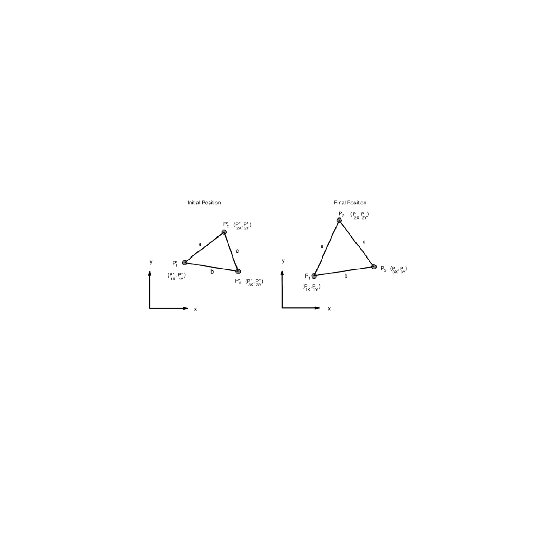
Measurement of the complete strain tensor is often achieved by examining three points placed in close

proximity.

7,82,111

For example, the Lagrangian strains on the surface of a tissue may be derived using the

relation.

– dS

= 2E

i, j = 1,2

(5.20)

where ds

is the deformed length, dS

is the undeformed length, and da

is the change in length in the

direction i. Letting P

′ and P

denote the initial and final positions of three points undergoing a general

planar deformation, as shown in

Figure 5.3

, the change in length of side a in the x-direction,

δa

, is given

δa

= (P

– P

) – (P

′ – P

′ )

(5.21)

and in the change in length in the y-direction,

δa

, is given by

δa

= (P

– P

) – (P

′ – P

′ )

(5.22)

The initial length of the side a, L

is given by

′ = (P

′ – P

′ )

+ (P

′ – P

′ )

)

1/2

(5.23)

FIGURE 5.3

Initial and final positions of three points forming a triangle on the surface of a body. Lagrangian

planar strains can be calculated directly from the initial and final lengths of the sides of the triangle.

and the deformed length of side a is given by

= ((P

– P

)

+ (P

– P

)

1/2

(5.24)

Applying Eq. 5.18 directly for side a, we obtain

– L

′

= 2E

(

δa

)

+ 4E

δa

+ 2E

(

δa

)

(5.25)

Using this approach for sides b and c results in three equations and the unknowns; L E

, E

, and E

can be solved for directly. Principal strains can be calculated solving the eigenvalue problem.

With tissue property and geometry variations, uniform loads give rise to nonhomogenous strain fields.

As a result, it often becomes necessary to determine the full-field strain distribution across the region of
interest in the tissue. Zerniche et al. found regional surface strains near the clamp during tendon testing
to be twice the value of strains in the middle of the test specimen. Further, tissue heterogeneity and the
presence of an active component in muscle imply, when measuring isometric strains in a muscle tendon
unit, that the strain within the structure may be changing. Van Bavel et al. simultaneously measured the
strains in both the aponeurosis and muscle belly of the rat medial gastrocnemius by tracking at least
three markers’ displacements in the region and by directly computing the Green-Lagrange strains.

108

Trestic and Lieber reported that this relative lengthening of passive structures and shortening within the
muscle belly resulted in 20% differences in predicted muscle force in the frog gastrocnemium.

106

Without

regional measurements of tendon, aponeurosis, and muscle strains in their experiment, these effects
might go unnoticed.

In an effort to improve accuracy and reduce noise in full-field strain measurement, investigators have

fitted the surface displacement across the entire tissue surface with a function and then differentiated
the function to attain the strain at each point.

8,97,101

Sutten et al. described a method which optimized

smoothing parameters to remove Gaussian noise on two-dimensional displacement data.

101

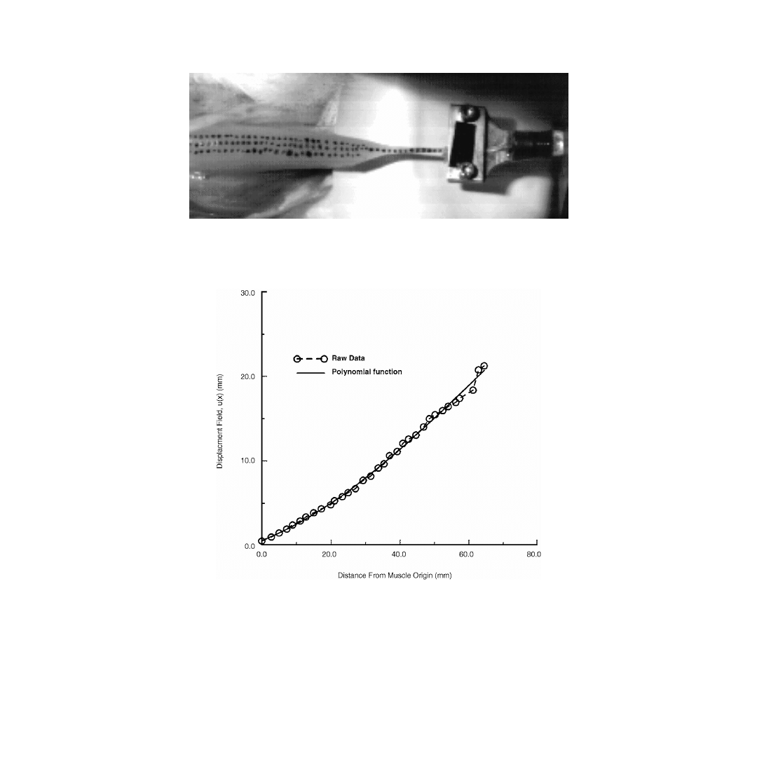
Best et al. fit

displacement data with a function to determine one-dimensional uniaxial finite strain in the rabbit tibialis
anterior.

Approximately 50 marks were stained along the muscle from origin to insertion (

Fig. 5.4

Image data were collected on a 1000 Hz, 238

× 192 pixel CCD camera. Axial deformation, u, vs. initial

position of the marker on the tissue, x, was digitized for each image, resulting in a complete u(x) history
(

Fig. 5.5

). Strain was calculated using the Lagrangian formulation (Eq. 5.15). While tensile axial defor-

mations of the muscle were large, transverse deformations and the change in transverse deformation
with respect to the initial position, x, were small. At maximum displacement, dv/dx was less than 0.06;
therefore, (dv/dx)

was less than 0.0036. Similarly, (dw/dx)

was less than 0.0009 at maximum displace-

ment. Therefore, the Eq. 5.15 was simplified to

(5.26)

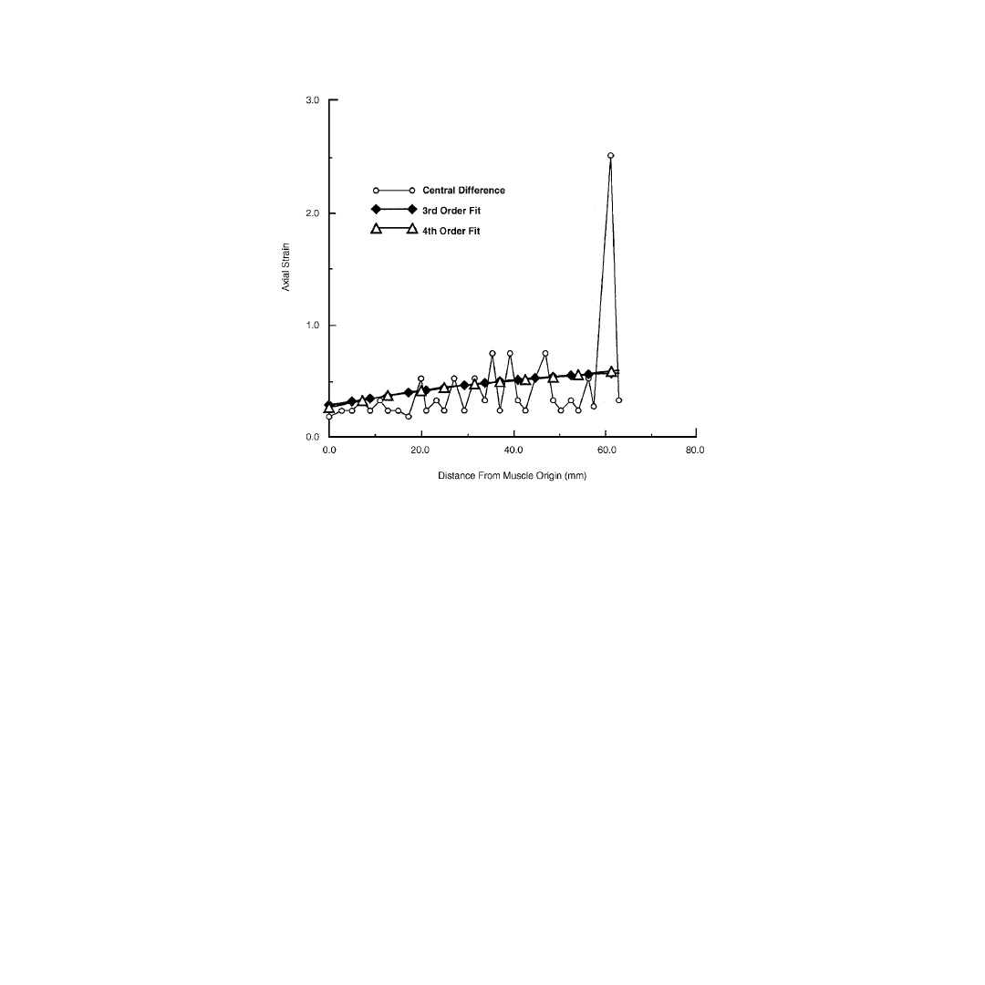
To illustrate the advantages obtained by fitting a continuous function to the displacement, derivatives of
the axial displacement, u(x), were determined by either a central difference method on the raw data or
by differentiation of a third or fourth order polynomial fit of the displacement data (

Fig. 5.6

). With this

particular model, the structure had a gauge length of 6 cm, and failed when elongated to 9 cm. Given
the limited spatial resolution of the imager, this resulted in a position resolution of approximately 0.5
mm/pixel. Strains calculated using a central difference method from the noisy, discretized data produced
errors on the order of the strain amplitude. Recognizing that discretization error is randomly distributed,
fitting a function to a set of points decreases error by 1/

where n is the number of points in the fitted

curve. In these experiments, this resulted in a decrease in error by a factor of 6.3. While splines tended
to have oscillations that produced negative strains when differentiated, polynomial functions were well-
behaved and were insensitive to the order of the polynomial (

Fig. 5.6

x, t

u t

( )

= ∂

( )

∂

( )

∂







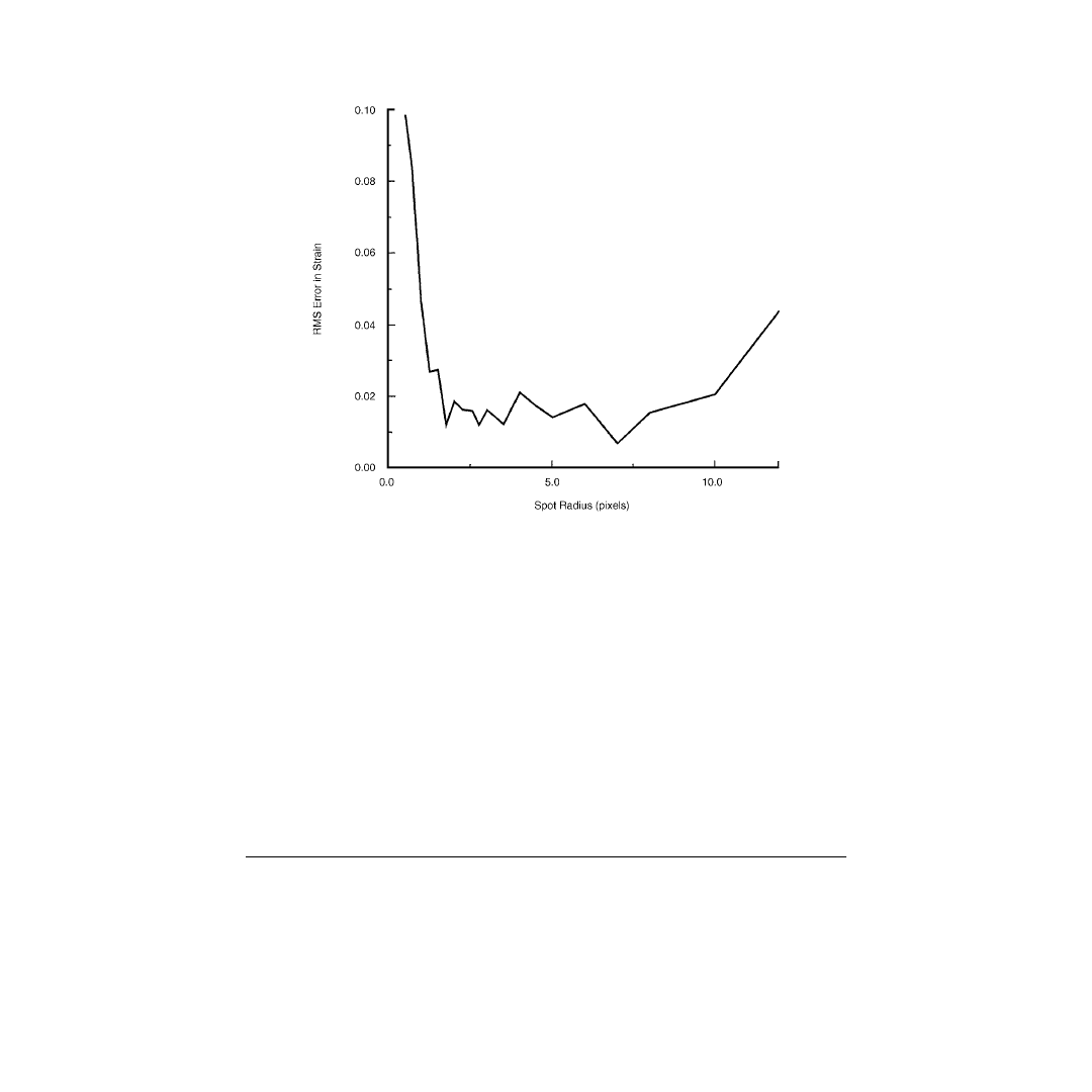
When fitting functions to multiple marker positions, a tradeoff between marker size and the number

of markers occurs. While both reduce error, increasing marker size decreases the number of marks which
can be placed on the surface. As the purpose of this technique is to minimize the error in the strain field
and not the position of each spot, it becomes necessary to optimize the benefits of larger spot size with
the benefits of greater numbers of spots. To that end, we generated numerical strain fields from previously
performed experiments to assess the effect of spot radii and number of spots on strain measurement

FIGURE 5.4

Digital image of the rabbit tibialis anterior with three sets of surface spots. The muscle origin is to

the right. The distal tendon, left, is inserted into the grip of a hydraulic actuator. Deflections in both the lateral and
axial directions were quantified by digitizing the black surface marks.

FIGURE 5.5

Discretized displacement of the surface markers on the rabbit tibialis anterior during passive elonga-

tion. These data illustrate the decrease in quantization error associated by fitting the displacement field with a
polynomial function.

accuracy. To determine the optimal spot size, a series of simulations was performed to emulate the CCD
camera’s data acquisition. Specifically, an algorithm was developed which placed a spot of a given radius
at a random location over the pixel array. Each pixel was then assigned a gray level from 0 to 255. Based
on a sample of 40 spots collected using this imaging system, the pixels completely covered by a spot were
assigned a gray level of 229 ± 9.6, and the pixels that were completely uncovered were assigned a
background gray level of 171 ± 6.0. Addition of the variation in pixel signal was found to profoundly
influence the results, illustrating the dependence of accuracy on the unique features of the particular
system under study. It also illustrates the need to calibrate and optimize each new experiment and test
system.

For those pixels partially covered by a spot, a Monte Carlo routine was developed to determine the

area fractions of spot and background. Gray level, GL, was then calculated based on the area fraction
occupied by the spot, f, the spot’s gray level, GI

, the area fraction occupied by the background, 1 – f,

and the background gray level, GL

, using the following equation:

GL = f · GI

+ (1 – f ) · GL

(5.27)

Defining accuracy as the RMS error in surface strain along the length of the muscle, the effects of spot
number vs. spot size were determined. Using this technique, we found that RMS strain error was
minimized over a range of spot radii from approximately 2 to 7 pixels (

Fig. 5.7

). Because of spot distortions

that occur in large spots in nonuniform strain fields, we suggest that the spot size chosen be toward the
smaller end of this range.

FIGURE 5.6 Axial strain calculated on the data from

Figure 5.5

using a central difference method, a third order,

and a fourth order polynomial to determine derivatives of the displacement field. The fitted curves are insensitive
to the order of the polynomial and reduce the effects of quantization error on calculated strain by an order of
magnitude.

Finite element analysis (FEA) has also been employed to determine nonhomogenous strain

fields.

5,38,46,53,76,83,119

Markers placed on the surface of the specimen serve as nodes for the finite elements.

The complete strain tensor can then be calculated at the Gauss points of the element. In addition, using
interpolation functions, strain distribution throughout the element can be calculated. Specific marker
placements need not be colinear nor regularly placed, and marker density can be increased in areas of
high strain variation. Finite element methods may be used in both planar and three-dimensional analyses.
Hoffman and Grigg used this method to determine strains within the posterior joint capsule of the cat
knee using planar linear elements.

Hashima et al. used a least squares method and bicubic Hermite

isoparametric elements to fit successive three-dimensional marker positions of the surface of a beating
canine heart.

Sutton et al. described a penalty method used in conjunction with FEA techniques to fit

noisy displacement data and determine strains.

101

Waldman and McCulloch investigated the effect of

random errors introduced by Gaussian noise on the calculated strain field, finding that the FEA method
reduced the errors in the strain field introduced by Gaussian noise by 50%.

113

5.5 Conclusion

Analysis of strain in muscle has evolved considerably. Beginning with average stretches measured by
simple transduction of actuator motion, to more complex and expensive optical measurement systems,
and progressing to full-field, three-dimensional large strain tensorial measurement systems based on
magnetic resonance and finite element techniques, the choices available to the investigator are vast.
Regardless of available resources, this review demonstrates the importance of proper definition of the
strain quantities to be determined and the importance of controlling the physiologic environment in
which the tissue deformation is measured. It also illustrates the need to carefully design the measurement
and data reduction strategy to quantify and minimize error. This is particularly true of optical systems,

FIGURE 5.7

RMS error in strain as a function of spot radius showing that error is minimized for pixel radii of

approximately 2 to 7 pixels.

in which contrast, variation in contrast, spot size, and other variables all influence system accuracy, and
the selection of the optimal system can only be achieved following careful experimental evaluation.

References

1. Adams, L.P., X-ray stereo photogrammetry locating the precise, three-dimensional positions of

image points, Med. Biol. Eng. Comput ., 19, 569, 1981.

2. Anderson, J.E., Carvalho, R.S., Yen, E., and Scott, J.E., Measurement of strain in cultured bone and

fetal muscle and lung cells, In Vitro Cell Dev. Biol ., 29A, 183, 1993.

3. Apter, J., Influence of composition on the thermal properties of tissues, in Biomechanics: Its

Foundations and Objectives , Fung, Y.C., Perrone, N., and Anliker, M., Eds., Prentice-Hall, Engle-
wood Cliffs, 1972, 217.

4. Arce, G.R. and McLoughlin, M.P., Theoretical analysis of the max/median filter, IEEE Trans. ASSP-

35, 1, 60, 1987.

5. Amodio, D., Broggiato, G.B., and Salvini, P., Finite strain analysis by image processing: smoothing

techniques, Strain , 31, 151, 1995.

6. Arms, S., Boyle, J., Johnson, R., and Pope, M., Strain measurement in the medial collateral ligament

of the human knee: an autopsy study, J. Biomechanics , 16, 491, 1983.

7. Barbee, K.A., Macarak, E.J., and Thibault, L.E., Strain measurements in cultured vascular smooth

muscle cells subjected to mechanical deformation, Ann. Biomed, Eng ., 22, 14, 1994.

8. Best, T.M., McElhaney, J.H., Garrett, W.E., Jr., and Myers, B.S., Axial strain measurements in skeletal

muscle at various strain rates, J. Biomechanical Eng ., 117, 262, 1995.

9. Brown, T.D., Sigal, L., Njus, G.O., Njus, N.M., Singerman, R.J., and Brand, R.A., Dynamic perfor-

mance characteristics of the liquid metal strain gage, J. Biomechanics , 19, 165, 1986.

10. Butler, D.L., Grood, E.S., Noyes, F.R., Zernicke, R.F., and Brackett, K., Effects of structure and

strain measurement technique on the material properties of young human tendons and fascia, J.
Biomechanics , 17, 579, 1984.

11. Butler, D.L., Noyes, F.R., and Grood, E.S., Measurements of the mechanical properties of ligaments,

in CRC Handbook of Engineering in Medicine and Biology , Fleming, D.V. and Feinberg, B.N., Eds.,
CRC Press, Cleveland, 1976, Sec. B.

12. Butler, D.L., Sheh, M.Y., Stouffer, D.C., Samaranayake, V.A., and Levy, M.S., Surface strain variation

in human patellar tendon and knee cruciate ligaments, Trans. ASME , 112, 38, 1990.

13. Butler, D.L. and Stouffer, D.C., Tension-torsion characteristics of the canine anterior cruciate

ligament II. Experimental observations, J. Biomechanical Eng ., 105, 160, 1983.

14. Chimich, D., Shrive, N., Frank, C., Marchuk, L., and Bray, R., Water content alters viscoelastic

behaviour of the normal adolescent rabbit medial collateral ligament, J. Biomechanics , 25, 831,
1992.

15. Cholewicki, J., Panjabi, M.M., Nibu, K., and Macias, M.E., Spinal ligament transducer based on a

Hall effect sensor, J. Biomechanics , 30, 291, 1997.

16. Chow, G.H., LeCroy, C.M., Seaber, A.V., Ribbeck, B.M., and Garrett, W.E., Sarcomere length and

maximal contractile force in rabbit skeletal muscle, J. Orthoped. Res., 8, 547, 1990.

17. Comninou, M. and Yannas, I.V., Dependence of stress-strain nonlinearity of connective tissues on

the geometry of collagen fibers, J. Biomechanics , 9, 427, 1976.

18. Crisp, J.D.C., Properties of tendon and skin, in Biomechanics: Its Foundations and Objectives ,

Fung, Y.C., Perrone, N., and Anliker, M., Eds., Prentice-Hall, Englewood Cliffs, 1972.

19. Cutts, A., The range of sarcomere lengths in the muscles of the human lower limb, J. Anat ., 160,

79, 1988.

20. De Clerck, N.M., Claes, V.A., Van Ocken, E.R., and Brutsaert, D.L., Sarcomere distribution patterns

in single cardiac cells, Biophys. J., 35, 237, 1981.

21. Demiray, H., A note on the elasticity of soft biological tissues, J. Biomechanics , 5, 309, 1972.

22. Derwin, K.A., Soslowsky, L.J., Green, W.D.K., and Elder, S.H., A new optical system for the

determination of deformations and strains: calibration characteristics and experimental results, J.
Biomechanics , 27, 1277, 1994.

23. Eastwood, A.B., Wood, D.S., Bock, K.L., and Sorenson, M.M., Chemically skinned mammalian

skeletal muscle I. The structure of skinned rabbit psoas, Tissue Cell , 11, 553, 1979.

24. Elmore, S.M., Sokoloff, L., and Carmeci, P., Nature of “imperfect” elasticity of articular cartilage,

J. Appl. Physiol ., 18, 393, 1963.

25. Figliola, R.S. and Beasley, D.E., Theory and Design for Mechanical Measurements , John Wiley &

Sons, New York, 1991.

26. Fitzgerald, E.R., Dynamic mechanical measurements during the life to death transition in animal

tissues, Biorheology, 12, 397, 1975.

27. Fitzgerald, E.R., Postmortem transition in the dynamic mechanical properties of bone, Medical

Phys., 4, 49, 1977.

28. Fleeter, T.B., Adams, P.J., Brenner, B., and Podolsky, R.J., A laser diffraction method for measuring

muscle sarcomere length in vivo for application to tendon transfers, J. Hand Surg . (U.S.), 10, 542,
1985.

29. Fung, Y.C., Foundations of Solid Mechanics , Prentice-Hall, Englewood Cliffs, 1965.
30. Galante, J.O., Tensile properties of the human annulus fibrosus, Acta Orthopaed. Scand . (suppl.),

100, 1, 1967.

31. Garrett, W.E., Jr., Nikolaou, P.K., Ribbeck, B.M., Glisson, R.R., and Seaber, A.V., The effect of

muscle architecture on the biomechanical failure properties of skeletal muscle under passive exten-
sion, Am. J. Sports Med ., 16, 7, 1988.

32. George, D.T. and Bogen, D.K., A low-cost fiber-optic strain gauge system for biological applications,

IEEE Trans. Biomed. Eng ., 38, 919, 1991.

33. Goldman, Y.E. and Simmons, R.M., Control of sarcomere length in skinned muscle fibres of Rana

temporaria during mechanical transients, J. Physiol. (London), 350, 497, 1984.

34. Goslow, G.E., Jr., Reinking, R.M., and Stuart, D.G., The cat step cycle: hind limb joint angles and

muscle lengths during unrestrained locomotion, J. Morphol., 141, 1, 1973.

35. Gottsauner-Wolf, F., Grabowski, J.J., Chao, E.Y., and An, K.N., Effects of freeze/thaw conditioning

on the tensile properties and failure mode of bone-muscle-bone units: a biomechanical and
histological study in dogs, J. Orthoped. Res ., 13, 90, 1995.

36. Graf, B.K., Vanderby, R., Jr., Ulm, M.J., Rogalski, R.P., and Thielke, R.J., Effect of preconditioning

on the viscoelastic response of primate patellar tendon, Arthroscopy , 10, 90, 1994.

37. Hardy, W.N., Foster, C.D., Tashman, S., and King, A.I., Current findings on the kinematics of brain

injury, in Injury Prevention through Biomechanics: Symposium Proceedings , Centers for Disease
Control, Atlanta, 1997, 137.

38. Hashima, A.R., Alistair, A.Y., McCulloch, A.D., and Waldman, L.K., Nonhomogeneous analysis of

epicardial strain distributions during acute myocardial ischemia in the dog, J. Biomechanics , 17,
795, 1993.

39. Haut, R.C., The influence of specimen length on the tensile failure properties of tendon collagen,

J. Biomechanics , 19, 951, 1986.

40. Haut, R.C. and Little, R.W., Rheological properties of canine anterior cruciate ligaments, J. Bio-

mechanics , 2, 289, 1969.

41. Haut, T.L. and Haut, R.C., The state of tissue hydration determines the strain-rate-sensitive stiffness

of human patellar tendon, J. Biomechanics , 30, 79, 1997.

42. Haut, R.C. and Powlison, A.C., The effects of test environment and cyclic stretching on the failure

properties of human patellar tendons, J. Orthoped. Res ., 8, 532, 1990.

43. Hawkins, D. and Bey, M., A comprehensive approach for studying muscle-tendon mechanics, J.

Biomechanical Eng ., 116, 51, 1994.

44. Hawkins, D.A., Gomez, M.A., and Woo, S.L.-Y., An indirect method to determine ligament stresses

in situ , ASME Adv. Bioeng ., 19, 166, 1986.

45. Heckman, J.L., Garvin, L., Brown, T., Stevenson-Smith, W., Santamore, W.P., and Lynch, P.R.,

Biplane ventriculography in the rat, Am. J. Physiol ., 250, H131, 1986.

46. Hoffman, A.H. and Griff, P., A method for measuring strains in soft tissue, J. Biomechanics , 26,

19, 1984.

47. Hughes, M.A., Myers, B.S., and Schenkman, M.L., The role of strength in rising from a chair in

the functionally impaired elderly, J. Biomechanics , 29, 1509, 1996.

48. James, M.R., Morris, W.L., and Cox, B.N., A high accuracy automated strain-field mapper, Exper-

imental Mech ., 60, March 1990.

49. Joshi, R.B., Bayoumi, A.E., and Zbib, H.M., The use of digital processing in studying stretch-

forming sheet metal, Experimental Mech ., 117, June 1992.

50. Kahn-Jetter, Z.L. and Chu, T.C., Three-dimensional displacement measurements using digital

image correlation and photogrammetric analysis, Experimental Mech ., 10, March 1990.

51. Kahn-Jetter, Z.L., Turso, J.A., and Pritchard, P.J., Deformed surface curve measurements using

photogrammetric techniques, Experimental Mech ., 43, January/February 1992.

52. Kearsley, E.A., Strain invariants expressed as average stretches, J. Rheology, 33, 757, 1989.
53. Kraitchman, D.L., Alistair, A.Y., Chang, C.N., and Axel, L., Semi-automatic tracking of myocardial

motion in MR tagged images, IEEE Trans. Medical Imaging , 14. 3. 1995.

54. Lai, W.M., Rubin, D., and Kermple, E., Introduction to Continuum Mechanics , Pergamon Press,

Tarrytown, NY, 1993.

55. Lam, T.C., Frank, C.B., and Shrive, N.G., Calibration characteristics of a video dimension analyser

(VDA) system, J. Biomechanics , 25, 1227, 1992.

56. Lanir, Y., A structural theory for the homogeneous biaxial stress-strain relationships in flat collag-

enous tissues, J. Biomechanics , 12, 423, 1979.

57. Lanir, Y., Constitutive equations for fibrous connective tissues, J. Biomechanics , 16, 1, 1983.
58. Leitschuh, P.H., Doherty, T.J., Taylor, D.C., Brooks, D.E., and Ryan, J.B., Effects of postmortem

freezing on tensile failure properties of rabbit extensor digitorum longus muscle-tendon complex,
J. Orthoped. Res ., 14, 830, 1996.

59. Lieber, R.L. and Friden, J., Muscle damage is not a function of muscle force but active muscle

strain, J. Appl. Physiol ., 74, 520, 1993.

60. Lieber, R.L., Leonard, M.E., Brown, C.G., and Trestik, C.L., Frog semitendinosis tendon load-strain

and stress-strain properties during passive loading, Am. J. Physiol ., 261, C86, 1991.

61. Lieber, R.L., Roos, K.P., Lubell, B.A., Cline, J.W., and Baskin, R.J., High-speed digital data acqui-

sition of sarcomere length from isolated skeletal and cardiac muscle cells, IEEE Trans. Biomed.
Eng., 30, 50, 1983.

62. Lieber, R.L., Yeh, Y., and Baskin, R.J., Sarcomere length determination using laser diffraction: effect

of beam and fiber diameter, Biophys. J., 45, 1007, 1984.

63. Lipscomb, K., Cardiac dimensional analysis by use of biplane cineradiography: description and

validation of method, Cathet. Cardiovasc. Diagn ., 6, 451, 1980.

64. Luo, P.f., Chao, Y.J., Sutton, M.A., and Peters, W.H., III, Accurate measurement of three dimensions

in deformable and rigid bodies using computer vision, Experimental Mech ., 123, June 1993.

65. Magid, A. and Law, D.J., Myofibrils bear most of the resting tension in frog skeletal muscle, Science ,

230, 1280, 1985.

66. McElhaney, J.H., Dynamic response of bone and muscle tissue, J. Appl. Physiol ., 21, 1231, 1966.
67. McElhaney, J.H., Paver, J.G., and McCrackin, H.J., Cervical spine compression responses, Paper

831615, Society of Automotive Engineers, 1983, 63.

68. Meglan, D., Berme, N., and Zuelzer, W., On the construction, circuitry and properties of liquid

metal strain gages, J. Biomechanics , 21, 681, 1988.

69. Meglan, D., Berme, N., Zuelzer, W., and Colvin, J., Direct measurement of anterior cruciate

ligament lengthening due to external loads, ASME Adv. Bioeng ., 19, 170, 1986.

70. Mendis, K.K., Stalnaker, R.L., and Advani, S.H., A constitutive relationship for large deformation

finite element modeling of brain tissue, J. Biomechanical Eng ., 117, 279, 1995.

71. Merrill, T., Goldsmith, W., and Deng, Y.C., Three-dimensional response of a lumped parameter

head-neck model due to impact and impulsive loading, J. Biomechanics , 17, 81, 1984.

72. Metz, C.E. and Fencil, L.E., Determination of three-dimensional structure in biplane radiography

without prior knowledge of the relationship between the two views: theory, Medical Phys ., 16, 45,
1989.

73. Miles, A.W. and Tanner, K.E., Strain Measurement in Biomechanics , Chapman & Hall, London,

1992.

74. Morgan, D.L., Claflin, D.R., and Julian, F.J., Tension as a function of sarcomere length and velocity

of shortening in single skeletal muscle fibres of the frog, J. Physiol. (London), 441, 719, 1991.

75. Moss, R.L., The effect of calcium on the maximum velocity of shortening in skinned skeletal muscle

fibres of the rabbit, J. Muscle Res. Cell Motility , 3, 295, 1982.

76. Moulton, J.M., Creswell, L.L., Actis, R.L., Myers, K.W., Vannier, M.W., Szabo, B.A., and Pasque,

M.K., An inverse approach to determining myocardial material properties, J. Biomechanics , 28,
935, 1995.

77. Myers, B.S., Woolley, C.T., Slotter, T.L., Garrett, W.E., and Best, T.M., Engineering stress-large

strain constitutive behavior of skeletal muscle, J. Biomechanical Eng ., 120(1), 126, 1998.

78. Natori, R., The property and contraction process of isolated myofibrils, Jikeikai Med. J., 1, 119, 1954.
79. Nightingale, R.W., McElhaney, J.H., Richardson, W.J., and Myers, B.S., Dynamic responses of the

head and cervical spine to axial impact loading, J. Biomechanics , 29, 307, 1996.

80. Noonan, T.J., Best, T.M., Seaber, A.V., and Garrett, W.E., Jr., Thermal effects on skeletal muscle

tensile behavior, Am. J. Sports Med ., 21, 517, 1993.

81. O’Dell, W.G., Moore, C.C., Hunter, W.C., Zerhouni, E.A., and McVeigh, E.R., Three-dimensional

myocardial deformations: calculation with displacement field fitting to tagged MR images, Radi-
ology, 195, 829, 1995.

82. Omens, J.H., MacKenna, D.A., and McCulloch, A.D., Measurement of strain and analysis of stress

in resting rat left ventricular myocardium, J. Biomechanics , 26, 665, 1993.

83. Oomens, C.W.J., Ratingen, M.R., Janssen, J.D., Kok, J.J., and Hendricks, M.A.N., A numerical-

experimental method for a mechanical characterization of biological materials, J. Biomechanics ,
26, 617, 1993.

84. Perng-Fei, G., Strain energy function for biological tissues, J. Biomechanics , 3, 547, 1970.
85. Prinzen, T.T., Arts, T., Prinzen, F.W., and Reneman, R.S., Mapping of epicardial deformation using

a video processing technique, J. Biomechanics , 19, 263, 1986.

86. Reuben, J.P., Brandt, P.W., Berman, M., and Grundfest, H., Regulation of tension in the skinned

crayfish muscle fiber I. Contraction and relaxation in the absence of Ca (pCa is greater than 9),
J. Gen. Physiol., 57, 385, 1971.

87. Reuben, J.P., Brandt, P.W., and Grundfest, H., Tension evoked in skinned crayfish muscle fibers by

anions, pH, and drugs, J. Gen. Physiol., 50, 250, 1967.

88. Riemersma, D.J. and Schamhaedt, H.C., The Cryo Jaw, a clamp designed for in vitro rheology

studies of horse digital flexor tendons, J. Biomechanics , 15, 619, 1982.

89. Riemersma, D.J. and van den Bogert, A.J., A method to estimate the initial length of equine tendons,

Acta Anat . (Basel), 146, 120, 1993.

90. Rigby, B.J., Hirai, N., Spikes, J.D., and Eyring, H., The mechanical properties of rat tail tendon, J.

Gen. Physiol ., 43, 265, 1959.

91. Sasaki, N. and Odajima, S., Elongation mechanism of collagen fibrils and force-strain relations of

tendon at each level of structural hierarchy, J. Biomechanics , 29, 1131, 1996.

92. Sasaki, N. and Odajima, S., Stress-strain curve and Young’s modulus of a collagen molecule as

determined by the X-ray diffraction technique, J. Biomechanics , 29, 655, 1996.

93. Schinagl, R.M., Ting, M.K., Price, J.H., Gough, D.A., and Sah, R.L., Video microscopy to quantitate

the inhomogeneous strain within articular cartilage during confined compression, ASME Adv.
Bioeng ., 26, 303, 1993.

94. Sevenhuijsen, P.J., Sirkis, J.S., and Bremand, F., Current trends in obtaining deformation data from

grids, Experimental Mech ., 22, May/June 1993.

95. Sharkey, N.A., Smith, T.S., and Lundmark, D.C., Freeze clamping musculo-tendinous junctions

for in vitro simulation of joint mechanics, J. Biomechanics , 28, 631, 1995.

96. Sirkis, J.S., System response to automated grid methods, Opt. Eng ., 29, 1485, 1990.
97. Sirkis, J.S. and Lim, T.J., Displacement and strain measurement with automated grid methods,

Experimental Mech ., 382, December 1991.

98. Smith, W.M. and Starmer, C.F., Error propagation in quantitative biplane cineroentgenography,

Phys. Med. Biol., 23, 677, 1978.

99. Smutz, W.P., Drexler, M., Berglund, E., Growney, E., and An, K.N., Accuracy of a video strain

measurement system, J. Biomechanics , 29, 813, 1996.

100. Stokes, I. and Greenapple, D.M., Measurement of surface deformation of soft tissue, J. Biomechan-

ics, 18, 1, 1985.

101. Sutton, M.A., Turner, J.L., Bruck, H.A., and Chae, T.A., Full-field representation of discretely

sampled surface deformation for displacement and strain analysis, Experimental Mech ., 168, June
1991.

102. Taylor, R.G., Geesink, G.H., Thompson, V.F., Koohmararie, M., and Goll, D.E., Is Z-disk degener-

ation responsible for postmortem tenderization? J. Anim. Sci ., 73, 1351, 1995.

103. Tencer, A.F. and Ahmed, A.M., The role of secondary variables in the measurement of the mechan-

ical properties of the lumbar intervertebral joint. J. Biomechanical Eng. , 103, 129, 1981.

104. Tidball, J.G. and Daniel, T.L., Elastic energy storage in rigored skeletal muscle cells under physio-

logical loading conditions, Am. J. Physiol ., 250, R56, 1986.

105. Tidball, J.G., Salem, G., and Zernicke, R., Site and mechanical conditions for failure of skeletal

muscle in experimental strain injuries, J. Appl. Physiol., 74, 1280, 1993.

106. Trestik, C.L. and Lieber, R.L., Relationship between Achilles tendon mechanical properties and

gastrocnemius muscle function, J. Biomechanical Eng ., 115, 225, 1993.

107. Valanis, K.C. and Landel, R.F., The strain-energy function of a hyperelastic material in terms of

the extension ratios, J. Appl. Phys., 38, 2997, 1967.

108. van Bavel, H., Drost, M.R., Wielders, J.D., Huyghe, J.M., Huson, A., and Janssen, J.D., Strain

distribution on rat medial gastrocnemium (MG) during passive stretch, J. Biomechanics , 29, 1069,
1996.

109. van Weeren, P.R., Jansen, M.O., van den Bogert, A.J., and Barneveld, A., A kinematic and strain

gauge study of the reciprocal apparatus in the equine hind limb., J. Biomechanics , 25, 1291, 1992.

110. Veronda, d.R. and Westman, R.A., Mechanical characterization of skin-finite deformations, J.

Biomechanics , 3, 111, 1970.

111. Villarreal, F.J., Waldman, L.K., and Lew, W.Y., Technique for measuring regional two-dimensional

finite strains in canine left ventricle, Circ. Res., 62, 711, 1988.

112. Waldman, L.K., Fung, Y.C., and Covell, J.W., Transmural myocardial deformation in the canine

left ventricle: normal in vivo three-dimensional finite strains, Circ. Res., 57, 152, 1985.

113. Waldman, L.K. and McCulloch, A.D., Nonhomogeneous ventricular wall strain: analysis of errors

and accuracy, J. Biomechanical Eng ., 115, 497, 1993.

114. Winter, D.A., Biomechanics and Motor Control of Human Movement , John Wiley & Sons, New

York, 1990.

115. Wollschlager, J., Lee, P., Zeiher, A., Solzbach, U., Bonzel, T., and Just, H., Derivation of spatial

information from biplane multidirectional coronary angiograms, Med. Prog. Technol ., 11, 57, 1986.

116. Woo, S.L.Y., An, K.N., Arnoczky, S.P., Wayne, J.S., Fithian, D.C., and Myers, B.S., Anatomy, biology,

and biomechanics of tendon, ligament, and meniscus, in Orthopaedic Basic Science , Simon, S.R.,
Ed., American Academy or Orthopaedic Surgeons, 1994.

117. Woo, S.L., Ritter, M.A., Amiel, D., Sanders, T.M., Gomez, M.A., Kuei, S.C., Garfin, S.R., and Akeson,

W.H., The biomechanical and biochemical properties of swine tendons: long-term effects of exer-
cise on the digital extensors, Connective Tissue Res ., 7, 177, 1980.

118. Yin, F.C., Tompkins, W.R., Peterson, K.L., and Intaglietta, M., A video-dimension analyzer, IEEE

Trans. Biomed. Eng ., 19, 376, 1972.

119. Young, A.A., Kraitchman, D.L., Dougherty, L., and Axel, L., Tracking and finite element analysis

of stripe deformation in magnetic resonance tagging, IEEE Trans. Medical Imaging , 14(3), 413,
1995.

120. Zajac, F.E., Muscle and tendon: properties, models, scaling, and application to biomechanics and

motor control, Crit. Rev. Biomed. Eng ., 17, 359, 1989.

121. Zernicke, R.F., Butler, D.L., Grood, E.S., and Hefzy, M.S., Strain topography of human tendon and

fascia, J. Biomechanical Eng ., 106, 177, 1984.

Document Outline

Musculoskeletal Models and Techniques
- Table of Contents
- Techniques and Applications for Strain Measurements of Skeletal Muscle

Wyszukiwarka

Podobne podstrony:
CH 05 UKORONOWANIE MARYI
CH 05 UKORONOWANIE MARYI
CH 05 UKORONOWANIE MARYI
Family in Transition Ch 05
Ethics ch 05
ch ćwicz 05
05 ch zapalne UN
06 04 05 kol 5 kwiet rozw ch
05 05 24 kol rozw ch
07 09 05 egz ch
9 Ch organiczna WĘGLOWODANY
podrecznik 2 18 03 05
regul praw stan wyjątk 05
ch wrzodowa prof T Starzyńska
05 Badanie diagnostyczneid 5649 ppt
Podstawy zarządzania wykład rozdział 05
ch zwyrodnieniowa st

więcej podobnych podstron