1

MESTREC notes.doc 12/2002 TDWC

1D NMR data processing with MESTREC

Introduction

The MESTREC NMR data processing software is designed to run on PC platforms only. The 1D
version of the program can display and manipulate single or multiple 1D spectra and allows for
detailed analysis and interpretation of NMR spectra. It is able to handle data formats from a wide
variety of instrument vendors and is able to automatically recognise and convert data to the
MESTREC format when opened. In all cases it is necessary to transfer the data from the spectrometer
onto the local processing station via the laboratory network.

These notes provide a brief introduction to the program and enable you to process, manipulate, store
and plot your data. Full “Help” manuals can be found on-line if you require further information or
wish to learn more about the program’s functionality.

All actions within MESTREC are executed with the mouse and the pull-down menus and many
functions can also be accessed with the icons on the upper toolbar. There is no command line for
typing in commands. Menu selections are indicated in bold italics in the following descriptions e.g.
File=Open to open a new data set.

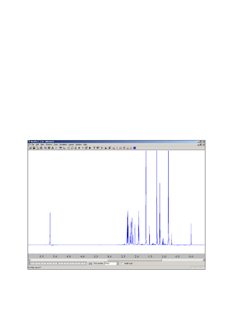
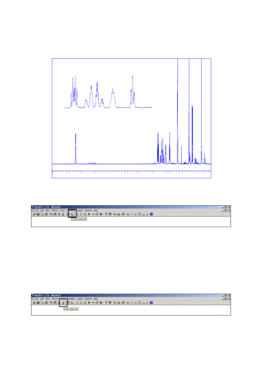
Figure 1: The MESTREC window.

2

Opening and importing files

Previously processed and saved MESTREC files can be recalled with the File=Open menu selection
and can be manipulated directly (by default MESTREC uses the .mrc three-letter extension for saved
files). Data taken directly from the spectrometers are opened in the same way and the program will
automatically determine the file type and translate this into the MESTREC format. Data from the
spectrometers are stored in a series of folders under the experiment name, which requires you to select
the raw FID named fid. THE MESTREC PROGRAM DOES NOT ALLOW YOU TO IMPORT
SPECTRA IN THE NATIVE SPECTROMETER FORMAT HENCE YOU MUST ALWAYS OPEN
THE RAW FID!

Raw data (FIDs) : Experiment name/experiment number/fid

Imported raw data requires additional manipulation prior to Fourier transformation but the program
determines what is required from the format of the raw data so no other pre-processing is required on
your part. The notable exception is the application of window functions (apodization), which must be
performed before the Fourier transform step described below (this is essential for heteronuclear
spectra where exponential multiplication is usually required, but is optional for proton spectra; see
Window functions below)

Fourier transformation

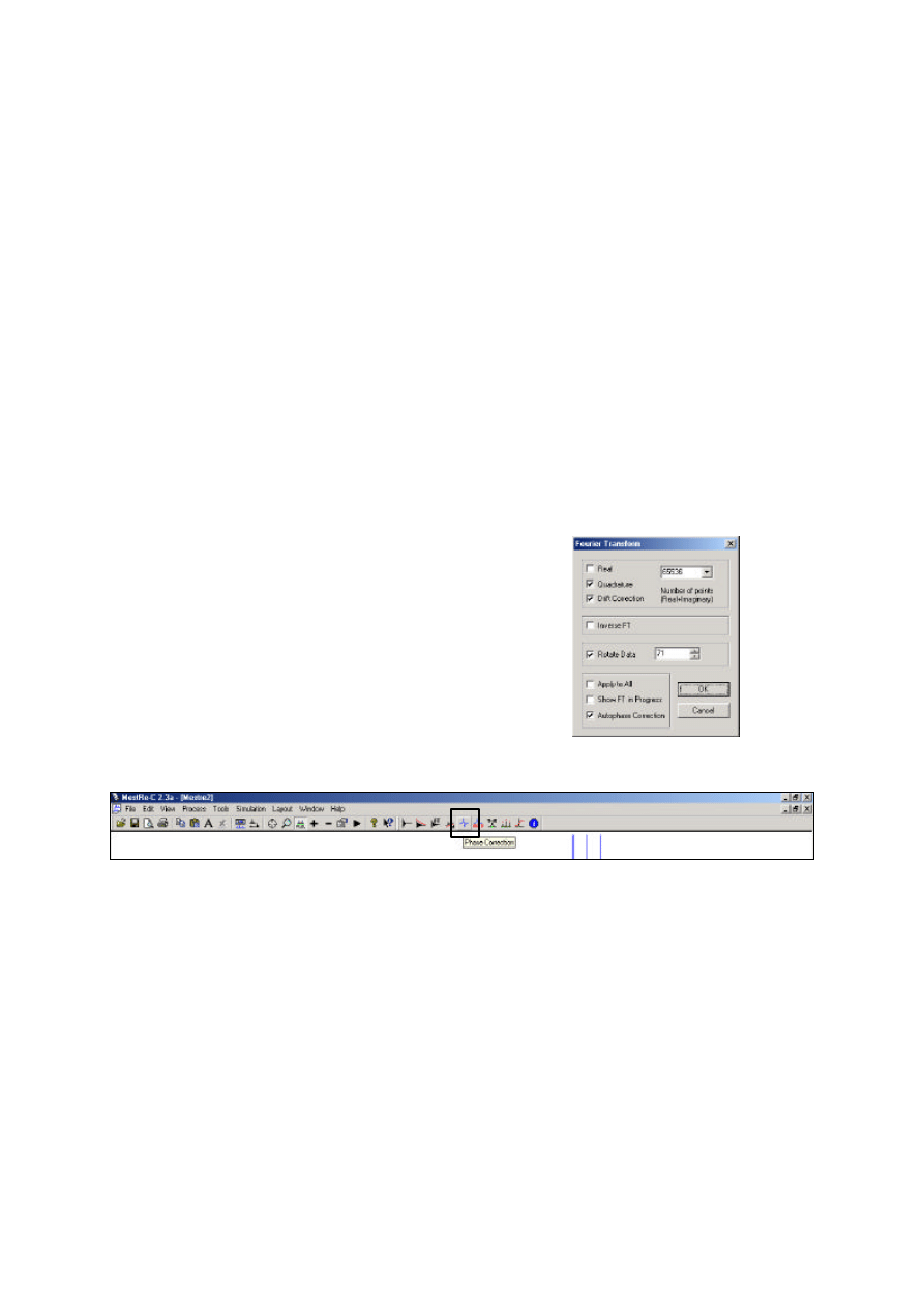
Phase correction

Automatic phase correction is usually accomplished with the above FT if Autophase Correction is
selected (see above). Occasionally some manual correction is also required which is activated with the
Phase Correction icon (or Process=Phase Correction). Use the Zero-Order correction to adjust the
phase of the left-most peak of the spectrum, then use the First-Order correction to adjust the right-most
peak. This should be sufficient to correct small phase errors.

Spectrum manipulation

Vertical scaling of the spectrum is made with the

+

and

–

icons on the tool bar. Horizontal scaling is

made within the Zoom tool (magnifying glass) which may be toggled on and off (or View=Zoom);
simply drag a box over the region of interest. The lower scroll bar may then be used for moving
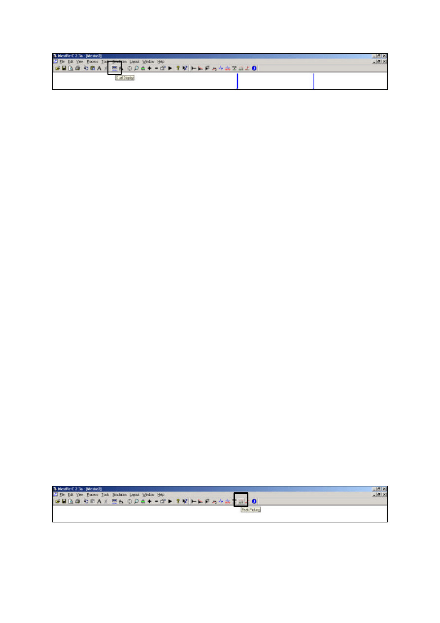
through the chemical shift range. An additional feature is the Dual display mode (View=Dual
Display) which may also be toggled on and off.

This is obviously only required if raw data has been opened for
the first time and may be achieved with the FT icon on the tool
bar (or Process=Fourier transform). You will be presented
with a parameter box describing details of the pre-processing
required; simply select OK to proceed and you should see a
correctly phased spectrum

3

In this mode the full spectrum is displayed above the expansion to help you navigate through the
spectrum whereby a greyed box indicates the currently viewed region. Moving or resizing the greyed
box of the dual display may also be used to alter the region seen in the main spectrum window.

To precisely define a chemical shift region to view use View=Set Limits and enter the high and low
shift values in the dialogue box.

The whole spectrum may be seen with the Full icon (or View=Full Spectrum). The spectrum baseline
position on the screen may be moved simply by clicking on the baseline at any point and dragging up
or down with the left mouse button.

Display properties, such as colours and axis fonts and details of the original spectrum acquisition
parameters (such as spectrometer frequency and spectrum title) can be accessed with the right mouse
button.

Calibration/referencing

To calibrate a spectrum first zoom in on the desired reference peak since this allows more accurate
results. Select the TMS icon (or Tools=Reference), place the cursor over the reference peak and click
left. A dialogue box appears in which you may enter the reference shift. Alternatively you may choose
from the predefined shift values for TMS or the residual solvent peak if appropriate.

Measuring Chemical shifts and J values

By holding down the mouse button a cross-hair cursor appears over the spectrum, beside which is
displayed the horizontal and vertical cursor position. Use this to accurately measure chemical shifts
and peak heights. To measure peak separations eg coupling constants, use the Tools=Measure
Coupling Constants feature. Place the cursor over the first multiplet line and left click; this defines the
reference peak from which others will be measured. Now move the cursor to an adjacent line and the
frequency difference in Hz will be displayed; clicking left again will add the J value to the text box
list. To delete the reference point, click on the right mouse button and repeat the above procedure to
measure other splittings. Stick diagrams may be added to the spectrum by selecting the appropriate
boxes in the Coupling Constants text window and this text may be copied and pasted into a text editor
such as Word, thus:

Shift 1

Shift 2

J(1-2)

1178.458

1172.783

5.675

1178.458

1169.946

8.512

1178.458

1167.108

11.350

1178.458

1164.271

14.187

1178.458

1158.596

19.862

Peak picking

Peak picking mode is activated with the Peak Picking icon (or Tools=Peak Picking=Peak Picking).

Now drag the cursor box over the regions to be picked, bearing in mind that the lower level of the box
defines the lower peak-picking threshold. Again the values are added to a text box which may be
edited if desired and can be copied and pasted, thus:

4

Point ppm

Hz

Height

----------------------------------------
*FROM* 40930 2.371 1185.709
*TO*

41148 2.302 1151.345

----------------------------------------
1

40976 2.356 1178.323

5.721

2

41012 2.345 1172.713

10.639

3

41030 2.339 1169.860

6.486

4

41048 2.334 1167.106

6.033

To see the peak picking on the spectrum, select Tools=Peak Picking=Options=Show Peak Picking on
Screen.

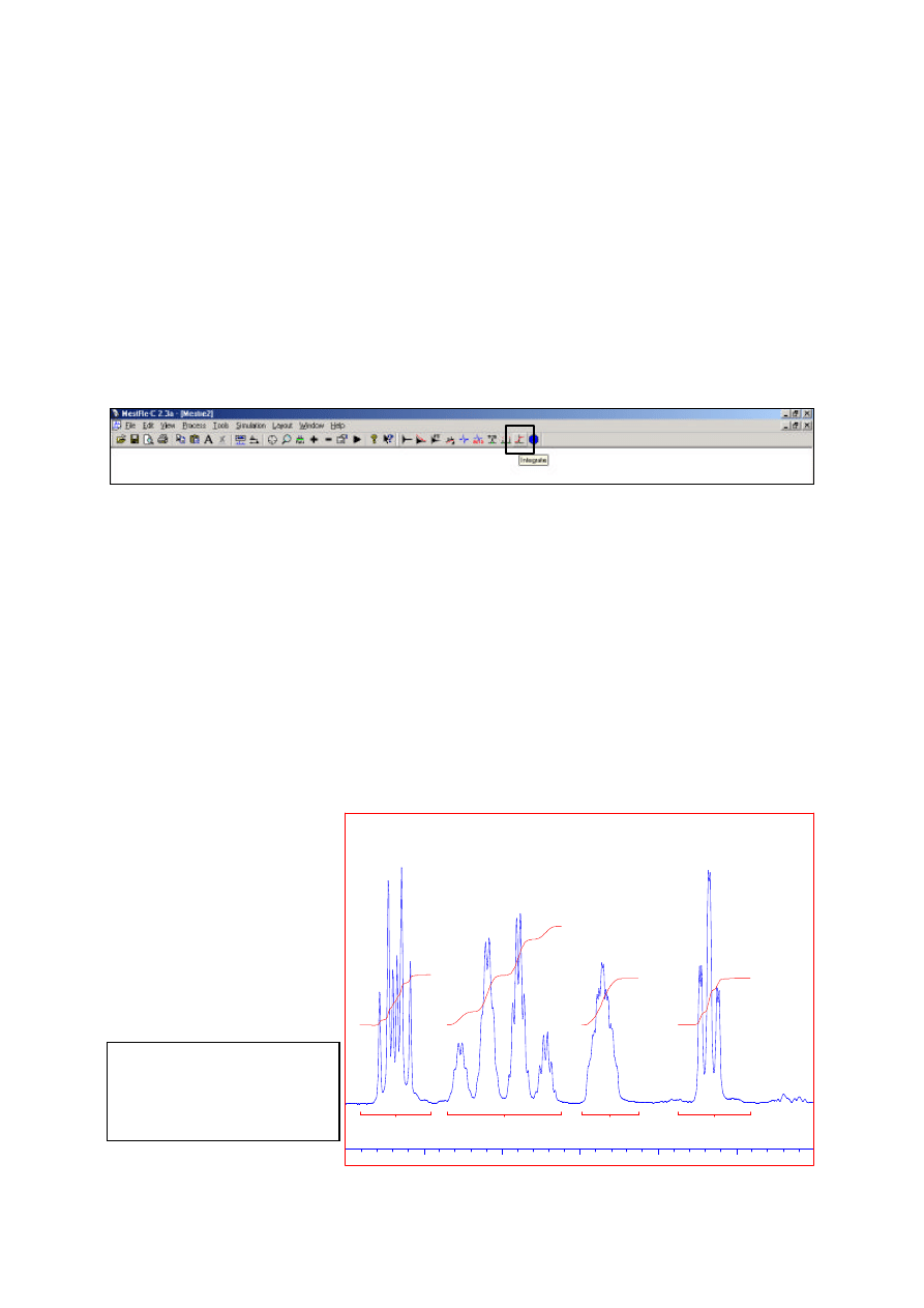
Integration

Select the Integration icon or use Tools=Integration=Integrate

As for peak picking, drag a box to define each integral region and then toggle out of the integrate
routine when all regions are defined. The size of each region may now be modified by clicking under
the integral trace which will produce a box that can be resized and repositioned above the spectrum.
Right clicking under a trace brings up a dialogue box in which the relative integral value (eg number
of protons) can be defined. The selected trace may also be deleted.

Integral display options, such as integral trails and labels on/off or label font and size can be altered
with Tools=Integration=integral options.

Plotting and copying

The program produces a plot equivalent to the current MESTREC screen display, including integrals,
peak-picking etc. The spectrum can also be copied from the screen (Edit=Copy) and pasted into other
documents e.g. Word or PowerPoint. One thing to watch here is the font sizes for the axis, peak
picking and integral labels which may appear too small when pasted. It is a good idea to increase the
font sizes (to 14-18 points) before copying the display.

1.90

2.00

2.10

2.20

2.30

1.0

2.0

0.9

0.9

Figure 2: A MESTREC

spectrum pasted into Word.

NB: the current program version
2.3a cannot correctly copy peak-
picking labels so it is advisable to
turn these off prior to copying and
pasting a spectrum.

5

Inset plots and labels

It is possible to plot multiple regions of the same spectrum on one plot, such as in fig. 3 below.

1.0

1.5

2.0

2.5

3.0

3.5

4.0

4.5

5.0

5.5

6.0

Expansion of 2.4 to 1.8 ppm

Figure 3: Additional expansions of the current spectrum.

This is accomplished by using the Create Expansion icon (or View=Create Expansion)

Firstly, display on the screen the region of the spectrum you wish to appear in the expansion window
using the usual zoom and scaling options as described above. When you are satisfied with the display,
select Create Expansion to add this region as an additional spectrum. This spectrum is now
considered the active spectrum (as indicated by the symbol on the far right of the spectrum baseline).
All manipulations now apply to the active spectrum only; simply click on the baseline of a spectrum to
define this as the active one or use the TAB key to jump between spectra (this also applies to the
multiple spectra display described below). The active frame can now be moved up and down on the
screen by dragging separately the baseline and the axes with the mouse. It may be moved and
expanded horizontally with the grey slider bar in the bottom left hand corner of the display. The active
spectrum may also be deleted with the Delete Spectrum icon (or Edit=Delete Spectrum)

Text labels may be added with the

A

text icon. Once created the text labels can be moved by drag and

drop and can be further edited by double-clicking on the text label. Other figures may also be pasted in
from the clipboard, such as ChemDraw structures, and moved and rescaled with the mouse.

6

Multiple Spectra

It is also possible to open a number of spectra simultaneously within the same window for direct
comparison. There are two options:

1. Add an additional spectrum to one already open with File=Open Additional Spectrum (the

new spectrum should already be saved in the MESTREC format before adding it to the
display)

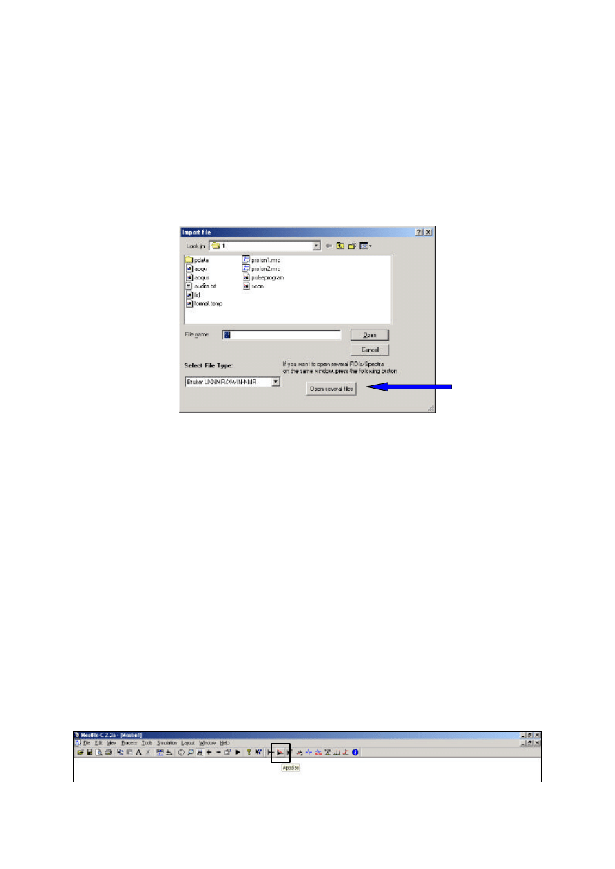
2. Use File=Open and select Open several files. Add the required files to the list and then Open.

Each spectrum is treated independently of the other with current manipulations performed only on the
active spectrum, as described above. To directly compare the same shift region select View=Zoom
options=Apply to all FIDs/Spectra and any zoom operations will apply simultaneously to all
displayed spectra. Alternatively define identical limits for each with View=Set Limits. Overlay plots
(each above the others) or stacked plots (each offset from the others) may be set up within the Layout
options.

Saving data

When imported your processed or raw data can be saved in MESTREC format for later retrieval. This
format stores all data in a single file which can have any name, but is given the .mrc extension by
default. It is sensible to keep separate copies of the original data transferred to the workstation (in case
you wish to use different processing parameters in the future) and that produced by MESTREC. You
are strongly encouraged to save all your data on ZIP or compact disks.

Window functions

Window functions can be used for enhancing spectrum features, such as sensitivity or resolution and
are discussed in more detail in the “Processing Techniques” handout. These must be applied to the raw
data (FID) before the FT and are usually essential for heteronuclear spectra eg carbon-13 but may also
be used to good effect in proton NMR, especially for resolution enhancement to better reveal multiplet
fine structure. To enter the window function mode use the Apodize icon (or Process=Apodize)

7

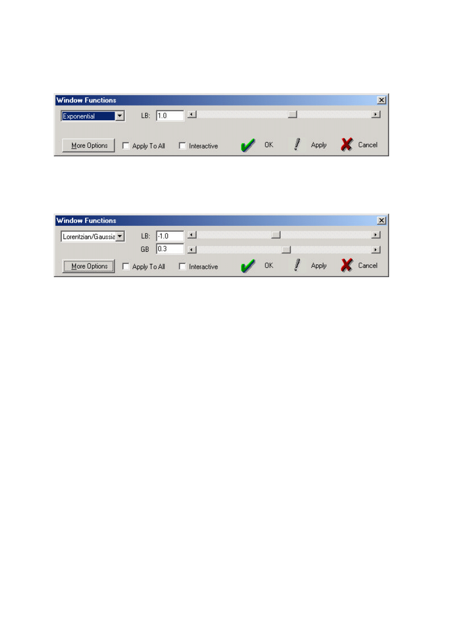
A second display of the FID will appear together with a line showing the shape of the window
function which is selected from the dialogue box:

Sensitivity enhancement uses the Exponential function and requires the LB (line broadening,

above) parameter to be set in Hz. (a typical value is 1 or 2 Hz for

13

C spectra). Select Apply and OK

to perform the exponential multiplication; the decay of the FID should be enhanced, which
corresponds to less noise but broader lines in the spectrum following FT.

Resolution enhancement uses the Lorentzian-Gaussian transformation which requires both

the LB and GB parameters to be set. LB is again set in Hz and defines the amount of line narrowing
(so must be a negative value) whilst GB defines the maximum of the Gaussian function and must be
between 0 and 1. Typical values for resolution enhancement of proton spectrum would be -1.0 and 0.3
respectively. This is executed with Apply and OK (Note: this is equivalent to the Bruker GM
function). Narrower lines should result in the spectrum following FT, along with a reduction in the
signal-to-noise level.

In general with window functions, it is a case of trial and error to get optimal results for your data,
especially when using resolution enhancement.

© Tim Claridge, Oxford, 2002