Filtry cyfrowe teoria

Digital Filter Design

By:

Douglas L. Jones

Digital Filter Design

By:

Douglas L. Jones

Online:

http://cnx.org/content/col10285/1.1/ >

C O N N E X I O N S

Rice University, Houston, Texas

This selection and arrangement of content is licensed under the Creative Commons Attribution License:
http://creativecommons.org/licenses/by/2.0/

Table of Contents

Overview of Digital Filter Design . . . . . . . . . . . . . . . . . . . . . . . . . . . . . . . . . . . . . . . . . . . . . . . . . . . . . . . . . . . . . . . . . . 1
1 FIR Filter Design

1.1 Linear Phase Filters . . . . . . . . . . . . . . . . . . . . . . . . . . . . . . . . . . . . . . . . . . . . . . . . . . . . . . . . . . . . . . . . . . . . . . . . . 3

1.2 Window Design Method . . . . . . . . . . . . . . . . . . . . . . . . . . . . . . . . . . . . . . . . . . . . . . . . . . . . . . . . . . . . . . . . . . . . . 7

1.3 Frequency Sampling Design Method for FIR lters . . . . . . . . . . . . . . . . . . . . . . . . . . . . . . . . . . . . . . . . . . . 9

1.4 Parks-McClellan FIR Filter Design . . . . . . . . . . . . . . . . . . . . . . . . . . . . . . . . . . . . . . . . . . . . . . . . . . . . . . . . . 11

1.5 Lagrange Interpolation . . . . . . . . . . . . . . . . . . . . . . . . . . . . . . . . . . . . . . . . . . . . . . . . . . . . . . . . . . . . . . . . . . . . . 18

Solutions . . . . . . . . . . . . . . . . . . . . . . . . . . . . . . . . . . . . . . . . . . . . . . . . . . . . . . . . . . . . . . . . . . . . . . . . . . . . . . . . . . . . . . . . 19

2 IIR Filter Design

2.1 Overview of IIR Filter Design . . . . . . . . . . . . . . . . . . . . . . . . . . . . . . . . . . . . . . . . . . . . . . . . . . . . . . . . . . . . . . 21

2.2 Prototype Analog Filter Design . . . . . . . . . . . . . . . . . . . . . . . . . . . . . . . . . . . . . . . . . . . . . . . . . . . . . . . . . . . . . 22

2.3 IIR Digital Filter Design via the Bilinear Transform . . . . . . . . . . . . . . . . . . . . . . . . . . . . . . . . . . . . . . . . 28

2.4 Impulse-Invariant Design . . . . . . . . . . . . . . . . . . . . . . . . . . . . . . . . . . . . . . . . . . . . . . . . . . . . . . . . . . . . . . . . . . . 32

2.5 Digital-to-Digital Frequency Transformations . . . . . . . . . . . . . . . . . . . . . . . . . . . . . . . . . . . . . . . . . . . . . . . 32

2.6 Prony's Method . . . . . . . . . . . . . . . . . . . . . . . . . . . . . . . . . . . . . . . . . . . . . . . . . . . . . . . . . . . . . . . . . . . . . . . . . . . . 33

2.7 Linear Prediction . . . . . . . . . . . . . . . . . . . . . . . . . . . . . . . . . . . . . . . . . . . . . . . . . . . . . . . . . . . . . . . . . . . . . . . . . . . 36

Solutions . . . . . . . . . . . . . . . . . . . . . . . . . . . . . . . . . . . . . . . . . . . . . . . . . . . . . . . . . . . . . . . . . . . . . . . . . . . . . . . . . . . . . . . . 39

Index . . . . . . . . . . . . . . . . . . . . . . . . . . . . . . . . . . . . . . . . . . . . . . . . . . . . . . . . . . . . . . . . . . . . . . . . . . . . . . . . . . . . . . . . . . . . . . . . 40

Attributions . . . . . . . . . . . . . . . . . . . . . . . . . . . . . . . . . . . . . . . . . . . . . . . . . . . . . . . . . . . . . . . . . . . . . . . . . . . . . . . . . . . . . . . . .41

Overview of Digital Filter Design

Advantages of FIR lters

1. Straight forward conceptually and simple to implement

2. Can be implemented with fast convolution

3. Always stable

4. Relatively insensitive to quantization

5. Can have linear phase (same time delay of all frequencies)

Advantages of IIR lters

1. Better for approximating analog systems

2. For a given magnitude response specication, IIR lters often require much less computation than an

equivalent FIR, particularly for narrow transition bands

Both FIR and IIR lters are very important in applications.
Generic Filter Design Procedure

1. Choose a desired response, based on application requirements

2. Choose a lter class

3. Choose a quality measure

4. Solve for the lter in class 2 optimizing criterion in 3

Perspective on FIR ltering

Most of the time, people do L

∞

optimal design, using the Parks-McClellan algorithm (Section 1.4). This

is probably the second most important technique in "classical" signal processing (after the Cooley-Tukey

(radix-2

) FFT).

Most of the time, FIR lters are designed to have linear phase. The most important advantage of FIR

lters over IIR lters is that they can have exactly linear phase. There are advanced design techniques for

minimum-phase lters, constrained L

optimal designs, etc. (see chapter 8 of text). However, if only the

magnitude of the response is important, IIR lers usually require much fewer operations and are typically

used, so the bulk of FIR lter design work has concentrated on linear phase designs.

This content is available online at <http://cnx.org/content/m12776/1.2/>.

"Decimation-in-time (DIT) Radix-2 FFT" <http://cnx.org/content/m12016/latest/>

Chapter 1

FIR Filter Design

1.1 Linear Phase Filters

In general, for −π ≤ ω ≤ π

H (ω) = |H (ω) |e

−(iθ(ω))

Strictly speaking, we say H (ω) is linear phase if

H (ω) = |H (ω) |e

−(iωK)

−(iθ

)

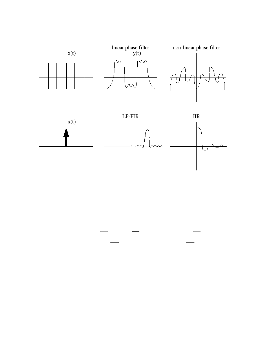
Why is this important? A linear phase response gives the same time delay for ALL frequencies! (Remember

the shift theorem.) This is very desirable in many applications, particularly when the appearance of the

time-domain waveform is of interest, such as in an oscilloscope. (see Figure 1.1)

This content is available online at <http://cnx.org/content/m12802/1.2/>.

CHAPTER 1. FIR FILTER DESIGN

Figure 1.1

1.1.1 Restrictions on h(n) to get linear phase

H (ω)

M −1
h=0

h (n) e

−(iωn)

h (0) + h (1) e

−(iω)

+ h (2) e

−(i2ω)

+ · · · +

h (M − 1) e

−(iω(M −1))

= e

−

(

iω

M −1

)

h (0) e

iω

M −1

+ · · · + h (M − 1) e

−

(

iω

M −1

)

−

(

iω

M −1

) (h (0) + h (M − 1)) cos

M −1

+ (h (1) + h (M − 2)) cos

M −3

+ · · · + i (h (0) − h (M − 1)) sin

M −1

+ . . .

(1.1)

For linear phase, we require the right side of (1.1) to be e

−(iθ

)

(real,positive function of ω). For θ

= 0

we thus require

h (0) + h (M − 1) =

real number

h (0) − h (M − 1) =

pure imaginary number

h (1) + h (M − 2) =

pure real number

h (1) − h (M − 2) =

pure imaginary number

...

Thus h (k) = h

∗

(M − 1 − k)

is a necessary condition for the right side of (1.1) to be real valued, for θ

= 0

For θ

, or e

−(iθ

)

= −i

, we require

h (0) + h (M − 1) =

pure imaginary

h (0) − h (M − 1) =

pure real number

...

⇒ h (k) = − (h

∗

(M − 1 − k))

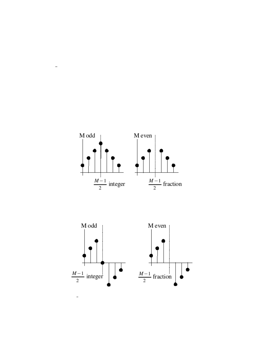
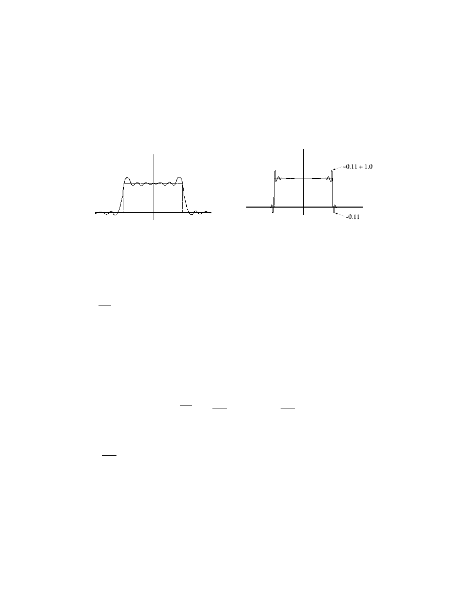
Usually, one is interested in lters with real-valued coecients, or see Figure 1.2 and Figure 1.3.

Figure 1.2: θ

= 0

(Symmetric Filters). h (k) = h (M − 1 − k).

Figure 1.3: θ

(Anti-Symmetric Filters). h (k) = − (h (M − 1 − k)).

CHAPTER 1. FIR FILTER DESIGN

Filter design techniques are usually slightly dierent for each of these four dierent lter types. We will

study the most common case, symmetric-odd length, in detail, and often leave the others for homework

or tests or for when one encounters them in practice. Even-symmetric lters are often used; the anti-

symmetric lters are rarely used in practice, except for special classes of lters, like dierentiators or Hilbert

transformers, in which the desired response is anti-symmetric.

So far, we have satised the condition that H (ω) = A (ω) e

−(iθ

)

−

(

iω

M −1

) where A (ω) is real-valued.

However, we have not assured that A (ω) is non-negative. In general, this makes the design techniques much

more dicult, so most FIR lter design methods actually design lters with Generalized Linear Phase:
H (ω) = A (ω) e

−

(

iω

M −1

), where A (ω) is real-valued, but possible negative. A (ω) is called the amplitude

of the frequency response.

excuse: A (ω) usually goes negative only in the stopband, and the stopband phase response is

generally unimportant.

note: |H (ω) | = ±A (ω) = A (ω) e

−

(

iπ

1
2

(1−signA(ω))

) where signx =







if x > 0

−1

if x < 0

Example 1.1

Lowpass Filter

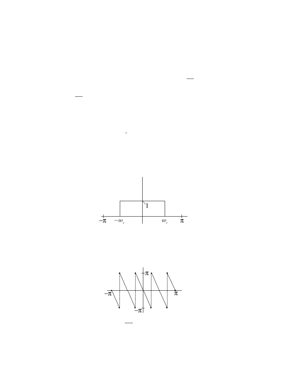
Desired |H(ω)|

Figure 1.4

Desired ∠H(ω)

Figure 1.5: The slope of each line is − `

M −1

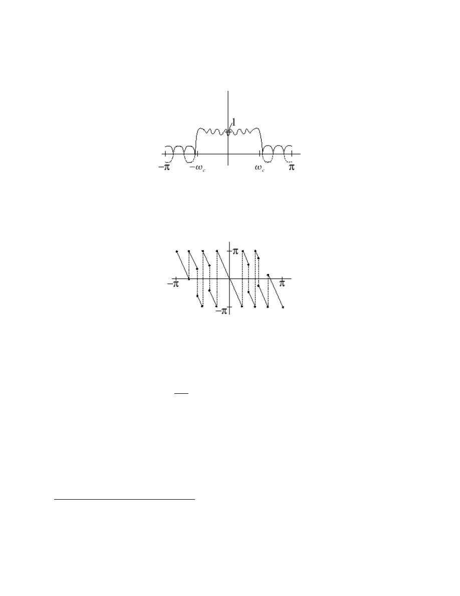
Actual |H(ω)|

Figure 1.6: A (ω) goes negative.

Actual ∠H(ω)

Figure 1.7: 2π phase jumps due to periodicity of phase. π phase jumps due to sign change in A (ω).

Time-delay introduces generalized linear phase.

note: For odd-length FIR lters, a linear-phase design procedure is equivalent to a zero-phase

design procedure followed by an

M −1

-sample delay of the impulse response

. For even-length lters,

the delay is non-integer, and the linear phase must be incorporated directly in the desired response!

1.2 Window Design Method

The truncate-and-delay design procedure is the simplest and most obvious FIR design procedure.

Exercise 1.1

(Solution on p. 19.)

Is it any Good?

"Impulse Response of a Linear System" <http://cnx.org/content/m12041/latest/>

This content is available online at <http://cnx.org/content/m12790/1.2/>.

CHAPTER 1. FIR FILTER DESIGN

1.2.1 L2 optimization criterion

nd ∀n, 0 ≤ n ≤ M − 1 : (h [n]), maximizing the energy dierence between the desired response and the

actual response: i.e., nd

min

h[n]

−π

(|H

(ω) − H (ω) |)

dω

by Parseval's relationship

min

h[n]

−π

(|H

(ω) − H (ω) |)

dω

2π

∞
n=−∞

(|h

[n] − h [n] |)

2π

−1
n=−∞

(|h

[n] − h [n] |)

+ P

M −1
n=0

(|h

[n] − h [n] |)

+ P

∞
n=M

(|h

[n] − h [n] |)

(1.2)

Since ∀n, n < 0n ≥ M : (= h [n]) this becomes

min

h[n]

−π

(|H

(ω) − H (ω) |)

dω

−1
h=−∞

(|h

[n] |)

M −1
n=0

(|h [n] − h

[n] |)

+ P

∞
n=M

(|h

[n] |)

Note: h [n] has no inuence on the rst and last sums.

The best we can do is let

h [n] =







[n]

if 0 ≤ n ≤ M − 1

if else

Thus h [n] = h

[n] w [n]

w [n] =







if 0 ≤ n (M − 1)

if else

is optimal in a least-total-sqaured-error ( L

, or energy) sense!

Exercise 1.2

(Solution on p. 19.)

Why, then, is this design often considered undersirable?

For desired spectra with discontinuities, the least-square designs are poor in a minimax (worst-case, or L

∞

)

error sense.

1.2.2 Window Design Method

Apply a more gradual truncation to reduce "ringing" (Gibb's Phenomenon

)

∀n0 ≤ n ≤ M − 1h [n] = h

[n] w [n]

Note: H (ω) = H

(ω) ∗ W (ω)

The window design procedure (except for the boxcar window) is ad-hoc and not optimal in any usual sense.

However, it is very simple, so it is sometimes used for "quick-and-dirty" designs of if the error criterion is

itself heurisitic.

"Parseval's Theorem" <http://cnx.org/content/m0047/latest/>

"Gibbs's Phenomena" <http://cnx.org/content/m10092/latest/>

1.3 Frequency Sampling Design Method for FIR lters

Given a desired frequency response, the frequency sampling design method designs a lter with a frequency

response exactly equal to the desired response at a particular set of frequencies ω

Procedure

∀k, k = [o, 1, . . . , N − 1] :

(ω

) =

M −1

n=0

h (n) e

−(iω

(1.3)

Note: Desired Response must incluce linear phase shift (if linear phase is desired)

Exercise 1.3

(Solution on p. 19.)

What is H

(ω)

for an ideal lowpass lter, coto at ω

Note: This set of linear equations can be written in matrix form

(ω

) =

M −1

n=0

h (n) e

−(iω

(1.4)










(ω

)

(ω

)

...

(ω

N −1

)



















−(iω

. . .

−(iω

(M −1))

−(iω

. . .

−(iω

(M −1))

...

−(iω

M −1

−(iω

M −1

. . .

−(iω

M −1

(M −1))



















h (0)

h (1)

...

h (M − 1)










(1.5)

= W h

h = W

−1

(1.6)

Note: W is a square matrix for N = M, and invertible as long as ω

6= ω

+ 2πl

, i 6= j

1.3.1 Important Special Case

What if the frequencies are equally spaced between 0 and 2π, i.e. ω

2πk

+ α

Then

(ω

) =

M −1

n=0

h (n) e

−

(

2πkn

−(iαn)

M −1

n=0

h (n) e

−(iαn)

−

(

2πkn

)

DFT!

h (n) e

−(iαn)

M −1

k=0

(ω

) e

2πnk

h [n] =

iαn

M −1

k=0

[ω

] e

2πnk

= e

iαn

IDF T [H

[ω

]]

This content is available online at <http://cnx.org/content/m12789/1.2/>.

CHAPTER 1. FIR FILTER DESIGN

1.3.2 Important Special Case #2

h [n]

symmetric, linear phase, and has real coecients. Since h [n] = h [−1], there are only

degrees of

freedom, and only

linear equations are required.

H [ω

]

M −1
n=0

h [n] e

−(iω







−1

n=0

h [n] e

−(iω

+ e

−(iω

(M −n−1))

if M even

M −

3
2

n=0

+h [n] e

−(iω

+ e

−(iω

(M −n−1))

M −1

−

(

iω

M −1

)

if M odd







−

(

iω

M −1

)2 P

−1

n=0

h [n] cos ω

M −1

− n

if M even

−

(

iω

M −1

)2 P

M −

3
2

n=0

h [n] cos ω

M −1

− n

+ h

M −1

if M odd

(1.7)

Removing linear phase from both sides yields

A (ω

) =







−1

n=0

h [n] cos ω

M −1

− n

if M even

M −

3
2

n=0

h [n] cos ω

M −1

− n

+ h

M −1

if M odd

Due to symmetry of response for real coecients, only

on ω ∈ [0, π) need be specied, with the

frequencies −ω

thereby being implicitly dened also. Thus we have

real-valued simultaneous linear

equations to solve for h [n].

1.3.2.1 Special Case 2a

h [n]

symmetric, odd length, linear phase, real coecients, and ω

equally spaced: ∀k, 0 ≤ k ≤ M − 1 :

nπk

h [n]

IDF T [H

(ω

)]

M −1
k=0

A (ω

) e

−

(

2πk

)

M −1

2πnk

M −1
k=0

A (k) e

(

2πk

(

n−

M −1

))

(1.8)

To yield real coecients, A (ω) mus be symmetric

A (ω) = A (−ω) ⇒ A [k] = A [M − k]

h [n]

A (0) +

M −1

k=1

A [k]

2πk

(

n−

M −1

) + e

−

(

i2πk

(

n−

M −1

))

A (0) + 2

M −1

k=1

A [k] cos

2πk

n −

M −1

A (0) + 2

M −1

k=1

A [k] (−1)

cos

2πk

n +

1
2

(1.9)

Simlar equations exist for even lengths, anti-symmetric, and α =

1
2

lter forms.

1.3.3 Comments on frequency-sampled design

This method is simple conceptually and very ecient for equally spaced samples, since h [n] can be computed

using the IDFT.

H (ω)

for a frequency sampled design goes exactly through the sample points, but it may be very far o

from the desired response for ω 6= ω

. This is the main problem with frequency sampled design.

Possible solution to this problem: specify more frequency samples than degrees of freedom, and minimize

the total error in the frequency response at all of these samples.

1.3.4 Extended frequency sample design

For the samples H (ω

)

where 0 ≤ k ≤ M − 1 and N > M, nd h [n], where 0 ≤ n ≤ M − 1 minimizing

k H

(ω

) − H (ω

) k

For k l k

∞

norm, this becomes a linear programming problem (standard packages availble!)

Here we will consider the k l k

norm.

To minimize the k l k

norm; that is, P

N −1
n=0

(|H

(ω

) − H (ω

) |)

, we have an overdetermined set of linear

equations:








−(iω

. . .

−(iω

(M −1))

...

−(iω

N −1

. . .

−(iω

N −1

(M −1))








h =










(ω

)

(ω

)

...

(ω

N −1

)










W h = H

The minimum error norm solution is well known to be h = W W

−1

W H

; W W

−1

is well known as

the pseudo-inverse matrix.

Note: Extended frequency sampled design discourages radical behavior of the frequency response

between samples for suciently closely spaced samples. However, the actual frequency response

may no longer pass exactly through any of the H

(ω

)

1.4 Parks-McClellan FIR Filter Design

The approximation tolerances for a lter are very often given in terms of the maximum, or worst-case,

deviation within frequency bands. For example, we might wish a lowpass lter in a (16-bit) CD player to

have no more than

1
2

-bit deviation in the pass and stop bands.

H (ω) =







1 −

≤ |H (ω) | ≤ 1 +

if |ω| ≤ ω

≥ |H (ω) |

if ω

≤ |ω| ≤ π

The Parks-McClellan lter design method eciently designs linear-phase FIR lters that are optimal in

terms of worst-case (minimax) error. Typically, we would like to have the shortest-length lter achieving

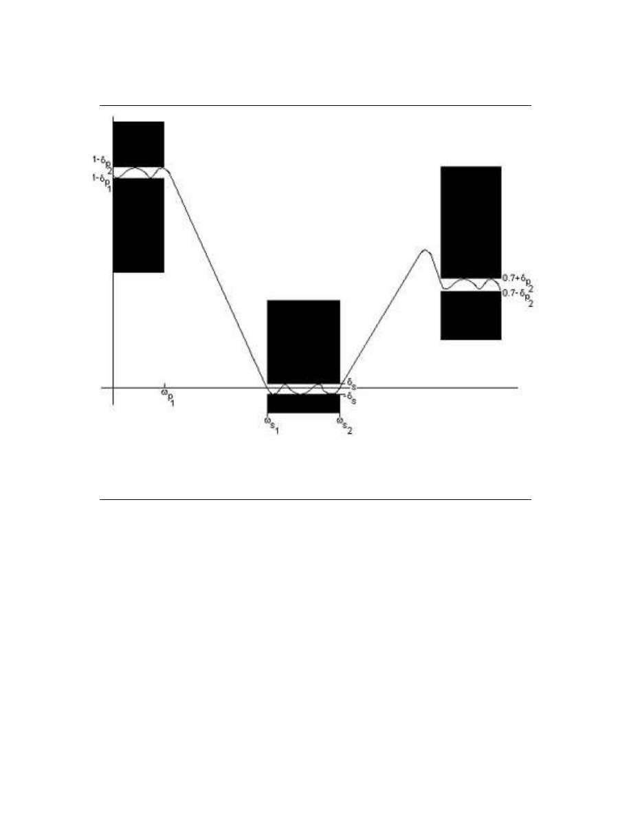
these specications. Figure Figure 1.8 illustrates the amplitude frequency response of such a lter.

This content is available online at <http://cnx.org/content/m12799/1.3/>.

CHAPTER 1. FIR FILTER DESIGN

Figure 1.8: The black boxes on the left and right are the passbands, the black boxes in the middle

represent the stop band, and the space between the boxes are the transition bands. Note that overshoots

may be allowed in the transition bands.

Exercise 1.4

(Solution on p. 19.)

Must there be a transition band?

1.4.1 Formal Statement of the L-∞ (Minimax) Design Problem

For a given lter length (M) and type (odd length, symmetric, linear phase, for example), and a relative

error weighting function W (ω), nd the lter coecients minimizing the maximum error

argmin

argmax

ω∈F

|E (ω) | = argmin

k E (ω) k

∞

where

E (ω) = W (ω) (H

(ω) − H (ω))

and F is a compact subset of ω ∈ [0, π] (i.e., all ω in the passbands and stop bands).

Note: Typically, we would often rather specify k E (ω) k

∞

≤ δ

and minimize over M and h;

however, the design techniques minimize δ for a given M. One then repeats the design procedure

for dierent M until the minimum M satisfying the requirements is found.

We will discuss in detail the design only of odd-length symmetric linear-phase FIR lters. Even-length

and anti-symmetric linear phase FIR lters are essentially the same except for a slightly dierent implicit

weighting function. For arbitrary phase, exactly optimal design procedures have only recently been developed

(1990).

1.4.2 Outline of L-∞ Filter Design

The Parks-McClellan method adopts an indirect method for nding the minimax-optimal lter coecients.

1. Using results from Approximation Theory, simple conditions for determining whether a given lter is

∞

(minimax) optimal are found.

2. An iterative method for nding a lter which satises these conditions (and which is thus optimal) is

developed.

That is, the L

∞

lter design problem is actually solved indirectly.

1.4.3 Conditions for L-∞ Optimality of a Linear-phase FIR Filter

All conditions are based on Chebyshev's "Alternation Theorem," a mathematical fact from polynomial

approximation theory.

1.4.3.1 Alternation Theorem
Let F be a compact subset on the real axis x, and let P (x) be and Lth-order polynomial

P (x) =

k=0

Also, let D (x) be a desired function of x that is continuous on F , and W (x) a positive, continuous weighting

function on F . Dene the error E (x) on F as

E (x) = W (x) (D (x) − P (x))

and

k E (x) k

∞

= argmax

x∈F

|E (x) |

A necessary and sucient condition that P (x) is the unique Lth-order polynomial minimizing k E (x) k

∞

that E (x) exhibits at least L + 2 "alternations;" that is, there must exist at least L + 2 values of x, x

∈ F

k = [0, 1, . . . , L + 1]

, such that x

< x

< · · · < x

L+2

and such that E (x

) = − (E (x

k+1

)) = ± (k E k

∞

)

Exercise 1.5

(Solution on p. 19.)

What does this have to do with linear-phase lter design?

1.4.4 Optimality Conditions for Even-length Symmetric Linear-phase Filters

For M even,

A (ω) =

n=0

h (L − n) cos

n +

where L =

− 1

Using the trigonometric identity cos (α + β) = cos (α − β) + 2cos (α) cos (β) to pull out

the

term and then using the other trig identities (p. 19), it can be shown that A (ω) can be written as

A (ω) = cos

k=0

cos

(ω)

CHAPTER 1. FIR FILTER DESIGN

Again, this is a polynomial in x = cos (ω), except for a weighting function out in front.

E (ω)

W (ω) (A

(ω) − A (ω))

W (ω) A

(ω) − cos

P (ω)

W (ω) cos

(ω)

cos

(

)

− P (ω)

(1.10)

which implies

E (x) = W

(x) A

(x) − P (x)

(1.11)

where

(x) = W

(cos (x))

−1

cos

(cos (x))

−1

and

(x) =

(cos (x))

−1

cos

1
2

(cos (x))

−1

Again, this is a polynomial approximation problem, so the alternation theorem holds. If E (ω) has at least
L + 2 =

+ 1

alternations, the even-length symmetric lter is optimal in an L

∞

sense.

The prototypical lter design problem:

W =







if |ω| ≤ ω

if |ω

| ≤ |ω|

See Figure 1.9.

Figure 1.9

1.4.5 L-∞ Optimal Lowpass Filter Design Lemma

1. The maximum possible number of alternations for a lowpass lter is L + 3: The proof is that the

extrema of a polynomial occur only where the derivative is zero:

∂

∂x

P (x) = 0

. Since P

(x)

is an

(L − 1)

th-order polynomial, it can have at most L − 1 zeros. However, the mapping x = cos (ω)

implies that

∂

∂ω

A (ω) = 0

at ω = 0 and ω = π, for two more possible alternation points. Finally, the

band edges can also be alternations, for a total of L − 1 + 2 + 2 = L + 3 possible alternations.

2. There must be an alternation at either ω = 0 or ω = π.

3. Alternations must occur at ω

and ω

. See Figure 1.9.

4. The lter must be equiripple except at possibly ω = 0 or ω = π. Again see Figure 1.9.

Note:

The alternation theorem doesn't directly suggest a method for computing the optimal

lter. It simply tells us how to recognize that a lter is optimal, or isn't optimal. What we need is

an intelligent way of guessing the optimal lter coecients.

CHAPTER 1. FIR FILTER DESIGN

In matrix form, these L + 2 simultaneous equations become

















cos (ω

)

cos (2ω

)

...

cos (Lω

)

W (ω

)

cos (ω

)

cos (2ω

)

...

cos (Lω

)

−1

W (ω

)

...

cos (ω

L+1

)

cos (2ω

L+1

)

...

cos (Lω

L+1

)

±1

W (ω

L+1

)
































h (L)

h (L − 1)

...

h (1)

h (0)
































(ω

)

(ω

)

...

(ω

L+1

)

























= A

So, for the given set of L + 2 extremal frequencies, we can solve for h and δ via (h, δ)

= W

−1

. Using the

FFT, we can compute A (ω) of h (n), on a dense set of frequencies. If the old ω

are, in fact the extremal

locations of A (ω), then the alternation theorem is satised and h (n) is optimal. If not, repeat the process

with the new extremal locations.

1.4.6 Computational Cost

O L

for the matrix inverse and Nlog

for the FFT (N ≥ 32L, typically), per iteration!

This method is expensive computationally due to the matrix inverse.

A more ecient variation of this method was developed by Parks and McClellan (1972), and is based on

the Remez exchange algorithm. To understand the Remez exchange algorithm, we rst need to understand

Lagrange Interpoloation.

Now A (ω) is an Lth-order polynomial in x = cos (ω), so Lagrange interpolation can be used to exactly

compute A (ω) from L + 1 samples of A (ω

)

, k = [0, 1, 2, ..., L].

Thus, given a set of extremal frequencies and knowing δ, samples of the amplitude response A (ω) can

be computed directly from the

A (ω

) =

(−1)

k(+1)

W (ω

)

δ + A

(ω

)

(1.12)

without solving for the lter coecients!

This leads to computational savings!

Note that (1.12) is a set of L + 2 simultaneous equations, which can be solved for δ to obtain (Rabiner,

1975)

δ =

L+1
k=0

(γ

(ω

))

L+1
k=0

(−1)

k(+1)

W (ω

)

(1.13)

where

L+1

i=0

i6=k

cos (ω

) − cos (ω

)

The result is the Parks-McClellan FIR lter design method, which is simply an application of the Remez

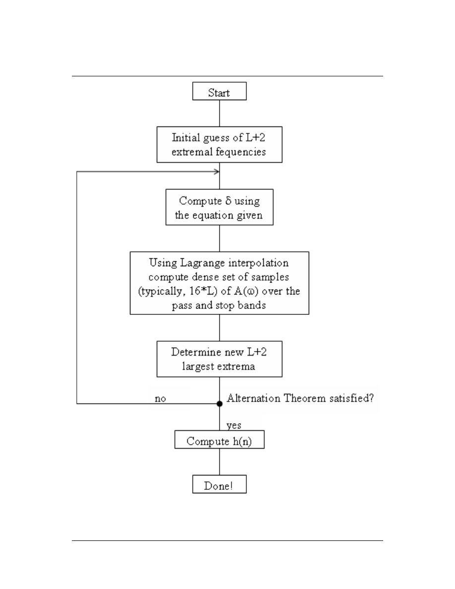
exchange algorithm to the lter design problem. See Figure 1.10.

Figure 1.10: The initial guess of extremal frequencies is usually equally spaced in the band. Computing
δ

costs O `L

. Using Lagrange interpolation costs O (16LL) ≈ O `16L

. Computing h (n) costs O `L

but it is only done once!

CHAPTER 1. FIR FILTER DESIGN

The cost per iteration is O 16L

, as opposed to O L

; much more ecient for large L. Can also

interpolate to DFT sample frequencies, take inverse FFT to get corresponding lter coecients, and zeropad

and take longer FFT to eciently interpolate.

1.5 Lagrange Interpolation

Lagrange's interpolation method is a simple and clever way of nding the unique Lth-order polynomial that

exactly passes through L + 1 distinct samples of a signal. Once the polynomial is known, its value can

easily be interpolated at any point using the polynomial equation. Lagrange interpolation is useful in many

applications, including Parks-McClellan FIR Filter Design (Section 1.4).

1.5.1 Lagrange interpolation formula

Given an Lth-order polynomial

P (x) = a

+ a

x + ... + a

k=0

and L + 1 values of P (x

)

at dierent x

, k ∈ {0, 1, ..., L}, x

6= x

, i 6= j, the polynomial can be written as

P (x) =

k=0

P (x

)

(x − x

) (x − x

) ... (x − x

k−1

) (x − x

k+1

) ... (x − x

)

− x

) (x

− x

) ... (x

− x

k−1

) (x

− x

k+1

) ... (x

− x

)

The value of this polynomial at other x can be computed via substitution into this formula, or by expanding

this formula to determine the polynomial coecients a

in standard form.

1.5.2 Proof

Note that for each term in the Lagrange interpolation formula above,

i=0,i6=k

x − x

− x







if x = x

∧ j 6= k

and that it is an Lth-order polynomial in x. The Lagrange interpolation formula is thus exactly equal to
P (x

)

at all x

, and as a sum of Lth-order polynomials is itself an Lth-order polynomial.

It can be shown that the Vandermonde matrix













...

... ...

... ... ...

...

























...

























P (x

)

P (x

)

P (x

)

...

P (x

)













has a non-zero determinant and is thus invertible, so the Lth-order polynomial passing through all L + 1

sample points x

is unique. Thus the Lagrange polynomial expressions, as an Lth-order polynomial passing

through the L + 1 sample points, must be the unique P (x).

This content is available online at <http://cnx.org/content/m12812/1.2/>.

http://en.wikipedia.org/wiki/Vandermonde_matrix

Solutions to Exercises in Chapter 1

Solution to Exercise 1.1 (p. 7)

Yes; in fact it's optimal! (in a certain sense)

Solution to Exercise 1.2 (p. 8): Gibbs Phenomenon

(a)

(b)

Figure 1.11: (a) A (ω), small M (b) A (ω), large M

Solution to Exercise 1.3 (p. 9)







−

(

iω

M −1

) if − ω

≤ ω ≤ ω

if − π ≤ ω < −ω

∨ ω

< ω ≤ π

Solution to Exercise 1.4 (p. 12)

Yes, when the desired response is discontinuous. Since the frequency response of a nite-length lter must

be continuous, without a transition band the worst-case error could be no less than half the discontinuity.
Solution to Exercise 1.5 (p. 13)

It's the same problem! To show that, consider an odd-length, symmetric linear phase lter.

H (ω)

M −1
n=0

h (n) e

−(iωn)

−

(

iω

M −1

)

M −1

+ 2 P

L
n=1

M −1

− n

cos (ωn)

(1.14)

A (ω) = h (L) + 2

n=1

(h (L − n) cos (ωn))

(1.15)

Where L

M −1

Using trigonometric identities (such as cos (nα) = 2cos ((n − 1) α) cos (α) − cos ((n − 2) α)), we can

rewrite A (ω) as

A (ω) = h (L) + 2

n=1

(h (L − n) cos (ωn)) =

k=0

cos

(ω)

where the α

are related to the h (n) by a linear transformation. Now, let x = cos (ω). This is a one-to-one

mapping from x ∈ [−1, 1] onto ω ∈ [0, π]. Thus A (ω) is an Lth-order polynomial in x = cos (ω)!

implication: The alternation theorem holds for the L

∞

lter design problem, too!

CHAPTER 1. FIR FILTER DESIGN

Therefore, to determine whether or not a length-M, odd-length, symmetric linear-phase lter is optimal in

an L

∞

sense, simply count the alternations in E (ω) = W (ω) (A

(ω) − A (ω))

in the pass and stop bands.

If there are L + 2 =

M +3

or more alternations, h (n), 0 ≤ n ≤ M − 1 is the optimal lter!

Chapter 2

IIR Filter Design

2.1 Overview of IIR Filter Design

2.1.1 IIR Filter

y (n) = −

M −1

k=1

y (n − k))

M −1

k=0

x (n − k))

H (z) =

+ b

−1

+ b

−2

+ ... + b

−M

1 + a

−1

+ a

−2

+ ... + a

−M

2.1.2 IIR Filter Design Problem

Choose {a

}

, {b

}

to best approximate some desired |H

(w) |

or, (occasionally), H

(w)

As before, dierent design techniques will be developed for dierent approximation criteria.

2.1.3 Outline of IIR Filter Design Material

•

Bilinear Transform - Maps k L k

∞

optimal (and other) analog lter designs to k L k

∞

optimal

digital IIR lter designs.

•

Prony's Method - Quasi-k L k

optimal method for time-domain tting of a desired impulse response

(ad hoc).

•

Lp Optimal Design - k L k

optimal lter design (1 < p < ∞) using non-linear optimization tech-

niques.

2.1.4 Comments on IIR Filter Design Methods

The bilinear transform method is used to design "typical" k L k

∞

magnitude optimal lters. The k L k

optimization procedures are used to design lters for which classical analog prototype solutions don't ex-

ist. The program by Deczky (DSP Programs Book, IEEE Press) is widely used. Prony/Linear Prediction

techniques are used often to obtain initial guesses, and are almost exclusively used in data modeling, system

identication, and most applications involving the tting of real data (for example, the impulse response of

an unknown lter).

This content is available online at <http://cnx.org/content/m12758/1.2/>.

CHAPTER 2. IIR FILTER DESIGN

2.2 Prototype Analog Filter Design

2.2.1 Analog Filter Design

Laplace transform:

H (s) =

∞

−∞

(t) e

−(st)

Note that the continuous-time Fourier transform

is H (iλ) (the Laplace transform evaluated on the imagi-

nary axis).

Since the early 1900's, there has been a lot of research on designing analog lters of the form

H (s) =

+ b

s + b

+ ... + b

1 + a

s + a

+ ... + a

A causal

IIR lter cannot have linear phase (no possible symmetry point), and design work for analog lters

has concentrated on designing lters with equiriplle (k L k

∞

) magnitude responses. These design problems

have been solved. We will not concern ourselves here with the design of the analog prototype lters, only

with how these designs are mapped to discrete-time while preserving optimality.

An analog lter with real coecients must have a magnitude response of the form

(|H (λ) |)

= B λ

H (iλ) H (iλ)

iλ+b

(iλ)

+...

1+a

iλ+a

(iλ)

+...

H (iλ)

−b

+...+iλ

(

−b

+...

)

1−a

+...+iλ(a

−a

+...)

−b

+...+iλ(b

−b

+...)

1−a

+...+iλ(a

−a

+...)

(

−b

+...

)

+λ

(

−b

+...

)

(1−a

+...)

+λ

−a

+...)

B λ

(2.1)

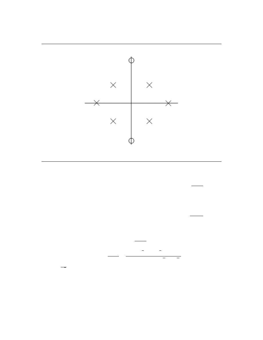
Let s = iλ, note that the poles and zeros of B − s

are symmetric around both the real and imaginary

axes: that is, a pole at p

implies poles at p

, p

, −p

, and − (p

)

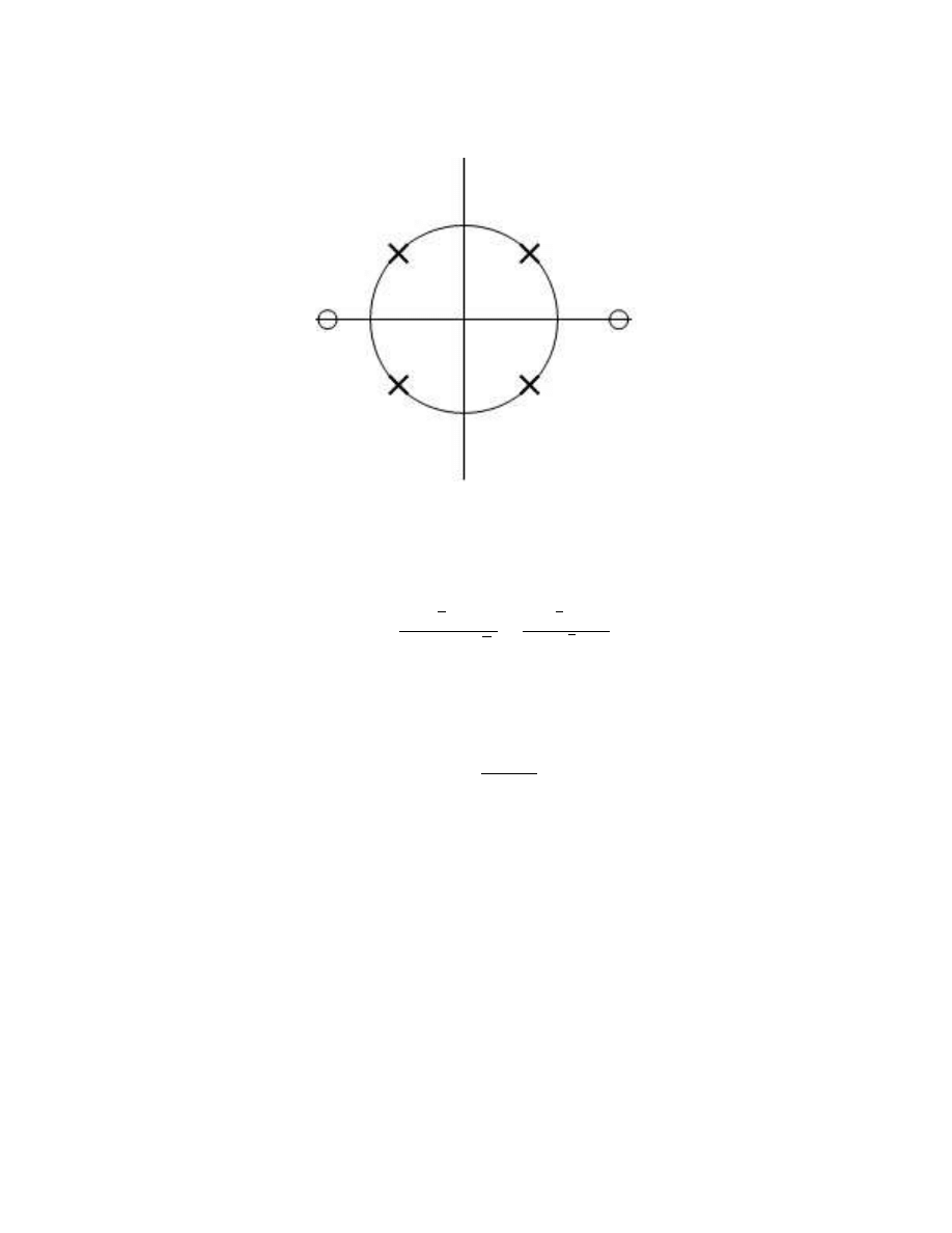
, as seen in Figure 2.1 (s-plane).

This content is available online at <http://cnx.org/content/m12763/1.2/>.

"Continuous-Time Fourier Transform (CTFT)" <http://cnx.org/content/m10098/latest/>

"Properties of Systems": Section Causality <http://cnx.org/content/m2102/latest/#causality>

s-plane

Figure 2.1

Recall that an analog lter is stable and causal if all the poles are in the left half-plane, LHP, and is

minimum phase if all zeros and poles are in the LHP.

s = iλ

: B λ

= B − s

= H (s) H (−s) = H (iλ) H (− (iλ)) = H (iλ) H (iλ)

we can factor

B − s

into H (s) H (−s), where H (s) has the left half plane poles and zeros, and H (−s) has the

RHP poles and zeros.

(|H (s) |)

= H (s) H (−s)

for s = iλ, so H (s) has the magnitude response B λ

. The trick to analog

lter design is to design a good B λ

, then factor this to obtain a lter with that magnitude response.

The traditional analog lter designs all take the form B λ

= (|H (λ) |)

1+F (λ

)

, where F is a

rational function in λ

Example 2.1

B λ

2 + λ

1 + λ

B − s

2 − s

1 + s

√

2 − s

√

2 + s

(s + α) (s − α) (s + α) (s − α)

where α =

1+i

√

Note: Roots of 1 + s

are N points equally spaced around the unit circle (Figure 2.2).

CHAPTER 2. IIR FILTER DESIGN

Figure 2.2

Take H (s) = LHP factors:

H (s) =

√

2 + s

(s + α) (s + α)

√

2 + s

√

2s + 1

2.2.2 Traditional Filter Designs

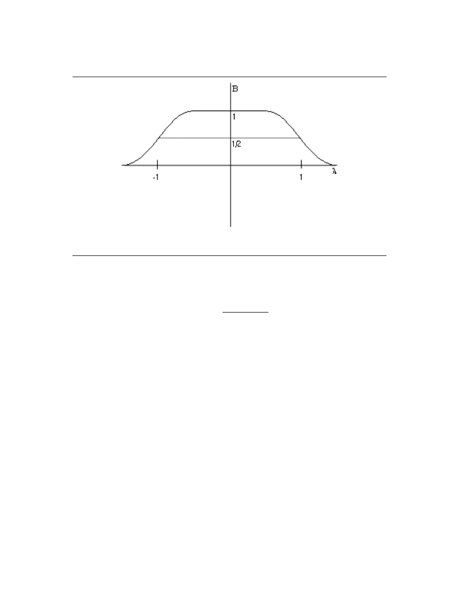
2.2.2.1 Butterworth

B λ

1 + λ

Note: Remember this for homework and rest problems!

"Maximally smooth" at λ = 0 and λ = ∞ (maximum possible number of zero derivatives). Figure 2.3.

B λ

= (|H (λ) |)

Figure 2.3

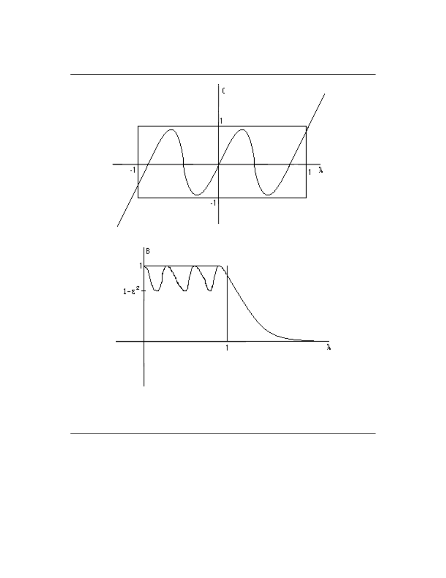
2.2.2.2 Chebyshev

B λ

1 +

(λ)

where C

(λ)

is an M

order Chebyshev polynomial. Figure 2.4.

CHAPTER 2. IIR FILTER DESIGN

(a)

(b)

Figure 2.4

2.2.2.3 Inverse Chebyshev
Figure 2.5.

Figure 2.5

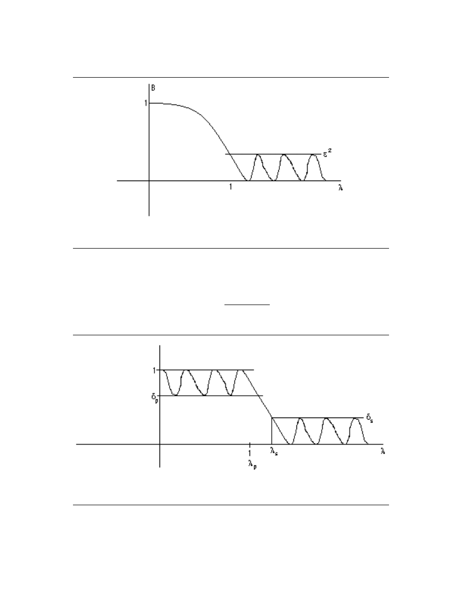
2.2.2.4 Elliptic Function Filter (Cauer Filter)

B λ

1 +

(λ)

where J

is the "Jacobi Elliptic Function." Figure 2.6.

Figure 2.6

The Cauer lter is k L k

∞

optimum in the sense that for a given M, δ

, δ

, and λ

, the transition

bandwidth is smallest.

CHAPTER 2. IIR FILTER DESIGN

That is, it is k L k

∞

optimal.

2.3 IIR Digital Filter Design via the Bilinear Transform

A bilinear transform maps an analog lter H

(s)

to a discrete-time lter H (z) of the same order.

If only we could somehow map these optimal analog lter designs to the digital world while preserving the

magnitude response characteristics, we could make use of the already-existing body of knowledge concerning

optimal analog lter design.

2.3.1 Bilinear Transformation

The Bilinear Transform is a nonlinear (C → C) mapping that maps a function of the complex variable s to

a function of a complex variable z. This map has the property that the LHP in s (< (s) < 0) maps to the

interior of the unit circle in z, and the iλ = s axis maps to the unit circle e

iω

in z.

Bilinear transform:

s = α

z − 1

z + 1

H (z) = H

s = α

z − 1

z + 1

Note:

iλ = α

iω

−1

iω

= α

(

iω

−1

)(

−(iω)

)

iω

+1)

(

−(iω)

)

2isin(ω)

2+2cos(ω)

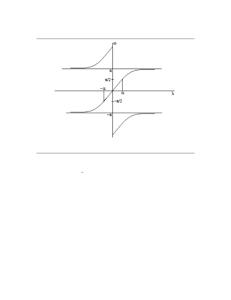
= iαtan

, so λ ≡ αtan

, ω ≡

2arctan

λ
α

. Figure 2.7.

This content is available online at <http://cnx.org/content/m12757/1.2/>.

Figure 2.7

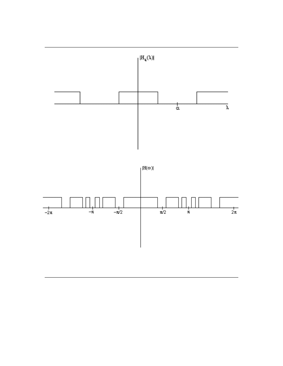
The magnitude response doesn't change in the mapping from λ to ω, it is simply warped nonlinearly

according to H (ω) = H

αtan

, Figure 2.8.

CHAPTER 2. IIR FILTER DESIGN

(a)

(b)

Figure 2.8: The rst image implies the second one.

Note: This mapping preserves k L k

∞

errors in (warped) frequency bands. Thus optimal Cauer

(k L k

∞

) lters in the analog realm can be mapped to k L k

∞

optimal discrete-time IIR lters

using the bilinear transform! This is how IIR lters with k L k

∞

optimal magnitude responses are

designed.

Note: The parameter α provides one degree of freedom which can be used to map a single λ

any desired ω

= αtan

α =

tan

This can be used, for example, to map the pass-band edge of a lowpass analog prototype lter to

any desired pass-band edge in ω. Often, analog prototype lters will be designed with λ = 1 as a

band edge, and α will be used to locate the band edge in ω. Thus an M

order optimal lowpass

analog lter prototype can be used to design any M

order discrete-time lowpass IIR lter with

the same ripple specications.

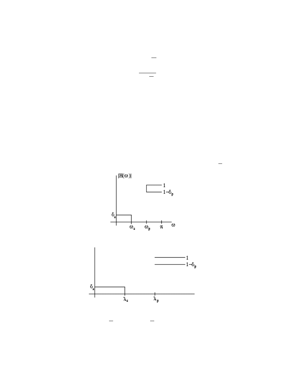
2.3.2 Prewarping

Given specications on the frequency response of an IIR lter to be designed, map these to specications in

the analog frequency domain which are equivalent. Then a satisfactory analog prototype can be designed

which, when transformed to discrete-time using the bilinear transformation, will meet the specications.

Example 2.2

The goal is to design a high-pass lter, ω

= ω

, ω

= ω

, δ

= δ

, δ

= δ

; pick up some α = α

In Figure 2.9 the δ

remain the same and the band edges are mapped by λ

= α

tan

(a)

(b)

Figure 2.9: Where λ

= α

tan

and λ

= α

tan

CHAPTER 2. IIR FILTER DESIGN

2.4 Impulse-Invariant Design

Pre-classical, adhoc-but-easy method of converting an analog prototype lter to a digital IIR lter. Does

not preserve any optimality.

Impulse invariance means that digital lter impulse response exactly equals samples of the analog proto-

type impulse response:

∀n : (h (n) = h

(nT ))

How is this done?

The impulse response of a causal, stable analog lter is simply a sum of decaying exponentials:

(s) =

+ b

s + b

+ ... + b

1 + a

s + a

+ ... + a

s − s

+ ... +

s − s

which implies

(t) = A

+ A

+ ... + A

u (t)

For impulse invariance, we desire

h (n) = h

(nT ) = A

+ A

+ ... + A

u (n)

Since

T )n

u (n) ≡

z − e

where |z| > |e

, and

H (z) =

k=1

z − e

where |z| > max

This technique is used occasionally in digital simulations of analog lters.

Exercise 2.1

(Solution on p. 39.)

What is the main problem/drawback with this design technique?

2.5 Digital-to-Digital Frequency Transformations

Given a prototype digital lter design, transformations similar to the bilinear transform can also be developed.

Requirements on such a mapping z

−1

= g z

−1

1. points inside the unit circle stay inside the unit circle (condition to preserve stability)

2. unit circle is mapped to itself (preserves frequency response)

This condition (list, item 2, p. 32) implies that e

−(iω

)

= g e

−(iω)

= |g (ω) |e

i∠(g(ω))

requires that

|g e

−(iω)

| = 1

on the unit circle!

Thus we require an all-pass transformation:

g z

−1

k=1

−1

− α

1 − α

−1

This content is available online at <http://cnx.org/content/m12760/1.2/>.

This content is available online at <http://cnx.org/content/m12759/1.2/>.

where |α

| < 1

, which is required to satisfy this condition (list, item 1, p. 32).

Example 2.3: Lowpass-to-Lowpass

−1

− a

1 − az

−1

which maps original lter with a cuto at ω

to a new lter with cuto ω

a =

sin

1
2

(ω

− ω

)

sin

1
2

(ω

+ ω

)

Example 2.4: Lowpass-to-Highpass

−1

+ a

1 + az

−1

which maps original lter with a cuto at ω

to a frequency reversed lter with cuto ω

a =

cos

1
2

(ω

− ω

)

cos

1
2

(ω

+ ω

)

(Interesting and occasionally useful!)

2.6 Prony's Method

Prony's Method is a quasi-least-squares time-domain IIR lter design method.

First, assume H (z) is an "all-pole" system:

H (z) =

1 +

M
k=1

−k

)

(2.2)

and

h (n) = −

k=1

h (n − k))

+ b

δ (n)

where h (n) = 0, n < 0 for a causal system.

Note: For h = 0, h (0) = b

Let's attempt to t a desired impulse response (let it be causal, although one can extend this technique when

it isn't) h

(n)

A true least-squares solution would attempt to minimize

∞

n=0

(|h

(n) − h (n) |)

where H (z) takes the form in (2.2). This is a dicult non-linear optimization problem which is known to

be plagued by local minima in the error surface. So instead of solving this dicult non-linear problem, we

solve the deterministic linear prediction problem, which is related to, but not the same as, the true

least-squares optimization.

The deterministic linear prediction problem is a linear least-squares optimization, which is easy to solve,

but it minimizes the prediction error, not the (|desired − actual|)

response error.

This content is available online at <http://cnx.org/content/m12762/1.2/>.

CHAPTER 2. IIR FILTER DESIGN

Notice that for n > 0, with the all-pole lter

h (n) = −

k=1

h (n − k))

(2.3)

the right hand side of this equation (2.3) is a linear predictor of h (n) in terms of the M previous samples

of h (n).

For the desired reponse h

(n)

, one can choose the recursive lter coecients a

to minimize the squared

prediction error

∞

n=1





(n) +

k=1

(n − k)) |





where, in practice, the ∞ is replaced by an N.

In matrix form, that's










(0)

...

(1)

(0)

...

(N − 1)

(N − 2)

...

(N − M )



















...










≈ −










(1)

(2)

...

(N )










a ≈ −h

The optimal solution is

= −

−1

Now suppose H (z) is an M

-order IIR (ARMA) system,

H (z) =

M
k=0

−k

1 +

M
k=1

−k

)

h (n)

−

M
k=1

h (n − k))

M
k=0

δ (n − k))







−

M
k=1

h (n − k))

+ b

if 0 ≤ n ≤ M

−

M
k=1

h (n − k))

if n > M

(2.4)

For n > M, this is just like the all-pole case, so we can solve for the best predictor coecients as before:










(M )

(M − 1)

...

(1)

(M + 1)

(M )

...

(2)

...

(N − 1)

(N − 2)

...

(N − M )



















...










≈










(M + 1)

(M + 2)

...

(N )










a ≈ ˆ

and

opt

−1

Having determined the a's, we can use them in (2.4) to obtain the b

's:

k=1

(n − k))

where h

(n − k) = 0

for n − k < 0.

For N = 2M, ˆ

is square, and we can solve exactly for the a

's with no error. The b

's are also chosen

such that there is no error in the rst M + 1 samples of h (n). Thus for N = 2M, the rst 2M + 1 points of
h (n)

exactly equal h

(n)

. This is called Prony's Method. Baron de Prony invented this in 1795.

For N > 2M, h

(n) = h (n)

for 0 ≤ n ≤ M, the prediction error is minimized for M + 1 < n ≤ N, and

whatever for n ≥ N + 1. This is called the Extended Prony Method.

One might prefer a method which tries to minimize an overall error with the numerator coecients,

rather than just using them to exactly t h

(0)

to h

(M )

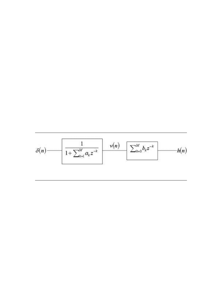
2.6.1 Shank's Method

1. Assume an all-pole model and t h

(n)

by minimizing the prediction error 1 ≤ n ≤ N.

2. Compute v (n), the impulse response of this all-pole lter.

3. Design an all-zero (MA, FIR) lter which ts v (n) ∗ h

(n) ≈ h

(n)

optimally in a least-squares sense

(Figure 2.10).

Figure 2.10: Here, h (n) ≈ h

(n)

The nal IIR lter is the cascade of the all-pole and all-zero lter.

This (list, item 3, p. 35) is is solved by

min







n=0





(n) −

k=0

v (n − k)) |











or in matrix form













v (0)

...

v (1)

v (0)

...

v (2)

v (1)

v (0)

...

v (N )

v (N − 1)

v (N − 2)

...

v (N − M )

























...













≈













(0)

(1)

(2)

...

(N )













CHAPTER 2. IIR FILTER DESIGN

Which has solution:

opt

= V

−1

Notice that none of these methods solve the true least-squares problem:

min

a,b

(

∞

n=0

(|h

(n) − h (n) |)

)

which is a dicult non-linear optimization problem. The true least-squares problem can be written as:

min

α,β







∞

n=0





(n) −

i=1











since the impulse response of an IIR lter is a sum of exponentials, and non-linear optimization is then used

to solve for the α

and β

2.7 Linear Prediction

Recall that for the all-pole design problem, we had the overdetermined set of linear equations:










(0)

...

(1)

(0)

...

(N − 1)

(N − 2)

...

(N − M )



















...










≈ −










(1)

(2)

...

(N )










with solution a = H

−1

Let's look more closely at H

= R

. r

is related to the correlation of h

with itself:

N −max{ i,j }

k=0

(k) h

(k + |i − j|))

Note also that:













(1)

(2)

(3)

...

(M )













where

(i) =

N −i

n=0

(n) h

(n + i))

so this takes the form a

opt

= − R

, or Ra = −r, where R is M × M, a is M × 1, and r is also M × 1.

This content is available online at <http://cnx.org/content/m12761/1.2/>.

Except for the changing endpoints of the sum, r

≈ r (i − j) = r (j − i)

. If we tweak the problem slightly

to make r

= r (i − j)

, we get:














r (0)

r (1)

r (2)

...

r (M − 1)

r (1)

r (0)

r (1)

...

r (2)

r (1)

r (0)

...

... ...

...

r (M − 1)

...

r (0)


























...













= −













r (1)

r (2)

r (3)

...

r (M )













The matrix R is Toeplitz (diagonal elements equal), and a can be solved for with O M

computations

using Levinson's recursion.

2.7.1 Statistical Linear Prediction

Used very often for forecasting (e.g. stock market).

Given a time-series y (n), assumed to be produced by an auto-regressive (AR) (all-pole) system:

y (n) = −

k=1

y (n − k))

+ u (n)

where u (n) is a white Gaussian noise sequence which is stationary and has zero mean.

To determine the model parameters {a

}

minimizing the variance of the prediction error, we seek

min

y (n) +

M
k=1

y (n − k))

= min

(n) + 2

M
k=1

y (n) y (n − k)) +

M
k=1

y (n − k))

M
l=1

y (n − l))

min

E [y

(n)] + 2

M
k=1

E [y (n) y (n − k)]) +

M
k=1

M
l=1

E [y (n − k) y (n − l)])

(2.5)

Note: The mean of y (n) is zero.

r (0)

r (1) r (2) r (3) ... r (M )













...













... a













r (0)

r (1) r (2)

...

r (M − 1)

r (1)

r (0) r (1)

...

r (2)

r (1) r (0)

...

... ...

...

r (M − 1)

...

r (0)













(2.6)

CHAPTER 2. IIR FILTER DESIGN

∂

∂a

= 2r + 2Ra

(2.7)

Setting (2.7) equal to zero yields: Ra = −r These are called the Yule-Walker equations. In practice, given

samples of a sequence y (n), we estimate r (n) as

r (n) =

N −n

k=0

(y (n) y (n + k)) ≈ E [y (k) y (n + k)]

which is extremely similar to the deterministic least-squares technique.

Solutions to Exercises in Chapter 2

Solution to Exercise 2.1 (p. 32)

Since it samples the non-bandlimited impulse response of the analog prototype lter, the frequency response

aliases. This distorts the original analog frequency and destroys any optimal frequency properties in the

resulting digital lter.

INDEX

Index of Keywords and Terms

Keywords are listed by the section with that keyword (page numbers are in parentheses). Keywords

do not necessarily appear in the text of the page. They are merely associated with that section. Ex.

apples, 1.1 (1) Terms are referenced by the page they appear on. Ex. apples, 1

alias, 2.4(32)

aliases, 39

all-pass, 32

amplitude of the frequency response, 6

bilinear transform, 28

design, 1.4(11)

deterministic linear prediction, 33

digital, 1.4(11)

DSP, 1.2(7), 1.3(9), 1.4(11)

Extended Prony Method, 35

lter, 1.3(9), 1.4(11)

lters, 1.2(7)

FIR, 1.2(7), 1.3(9), 1.4(11)

FIR lter, (1)

FIR lter design, 1.1(3)

Generalized Linear Phase, 6

IIR Filter, (1)

interpolation, 1.5(18)

lagrange, 1.5(18)

linear predictor, 34

minimum phase, 23

optimal, 16

polynomial, 1.5(18)

pre-classical, 2.4(32), 32

Prony's Method, 35

Toeplitz, 37

Yule-Walker, 38

ATTRIBUTIONS

Attributions

Collection: Digital Filter Design

Edited by: Douglas L. Jones

URL: http://cnx.org/content/col10285/1.1/

License: http://creativecommons.org/licenses/by/2.0/
Module: "Overview of Digital Filter Design"

By: Douglas L. Jones

URL: http://cnx.org/content/m12776/1.2/

Pages: 1-1

License: http://creativecommons.org/licenses/by/2.0/
Module: "Linear Phase Filters"

By: Douglas L. Jones

URL: http://cnx.org/content/m12802/1.2/

Pages: 3-7

License: http://creativecommons.org/licenses/by/2.0/
Module: "Window Design Method"

By: Douglas L. Jones

URL: http://cnx.org/content/m12790/1.2/

Pages: 7-8

License: http://creativecommons.org/licenses/by/2.0/
Module: "Frequency Sampling Design Method for FIR lters"

By: Douglas L. Jones

URL: http://cnx.org/content/m12789/1.2/

Pages: 9-11

License: http://creativecommons.org/licenses/by/2.0/
Module: "Parks-McClellan FIR Filter Design"

By: Douglas L. Jones

URL: http://cnx.org/content/m12799/1.3/

Pages: 11-18

License: http://creativecommons.org/licenses/by/2.0/
Module: "Lagrange Interpolation"

By: Douglas L. Jones

URL: http://cnx.org/content/m12812/1.2/

Pages: 18-18

License: http://creativecommons.org/licenses/by/2.0/

ATTRIBUTIONS

Module: "Overview of IIR Filter Design"

By: Douglas L. Jones

URL: http://cnx.org/content/m12758/1.2/

Pages: 21-21

License: http://creativecommons.org/licenses/by/2.0/
Module: "Prototype Analog Filter Design"

By: Douglas L. Jones

URL: http://cnx.org/content/m12763/1.2/

Pages: 22-28

License: http://creativecommons.org/licenses/by/2.0/
Module: "IIR Digital Filter Design via the Bilinear Transform"

By: Douglas L. Jones

URL: http://cnx.org/content/m12757/1.2/

Pages: 28-32

License: http://creativecommons.org/licenses/by/2.0/
Module: "Impulse-Invariant Design"

By: Douglas L. Jones

URL: http://cnx.org/content/m12760/1.2/

Pages: 32-32

License: http://creativecommons.org/licenses/by/2.0/
Module: "Digital-to-Digital Frequency Transformations"

By: Douglas L. Jones

URL: http://cnx.org/content/m12759/1.2/

Pages: 32-33

License: http://creativecommons.org/licenses/by/2.0/
Module: "Prony's Method"

By: Douglas L. Jones

URL: http://cnx.org/content/m12762/1.2/

Pages: 33-36

License: http://creativecommons.org/licenses/by/2.0/
Module: "Linear Prediction"

By: Douglas L. Jones

URL: http://cnx.org/content/m12761/1.2/

Pages: 36-38

License: http://creativecommons.org/licenses/by/2.0/

Digital Filter Design

An electrical engineering course on digital lter design.

About Connexions

Since 1999, Connexions has been pioneering a global system where anyone can create course materials and

make them fully accessible and easily reusable free of charge. We are a Web-based authoring, teaching and

learning environment open to anyone interested in education, including students, teachers, professors and

lifelong learners. We connect ideas and facilitate educational communities.
Connexions's modular, interactive courses are in use worldwide by universities, community colleges, K-12

schools, distance learners, and lifelong learners. Connexions materials are in many languages, including

English, Spanish, Chinese, Japanese, Italian, Vietnamese, French, Portuguese, and Thai. Connexions is part

of an exciting new information distribution system that allows for Print on Demand Books. Connexions

has partnered with innovative on-demand publisher QOOP to accelerate the delivery of printed course

materials and textbooks into classrooms worldwide at lower prices than traditional academic publishers.

Wyszukiwarka

Podobne podstrony:
koszałka,teoria sygnałów, Filtry cyfrowe
FILTRY CYFROWE1
filtry cyfrowe
asb filtry cyfrowe 7
filtry cyfrowe id 171064 Nieznany
filtry cyfrowe, CPS8, Ćwiczenie
filtry cyfrowe, Akademia Morska -materiały mechaniczne, szkoła, GRZES SZKOLA, szkoła, automaty, ayto
Wyklad Filtry cyfrowe1
Filtry RC teoria
filtry cyfrowe, CPS7, Ćw
filtry cyfrowe, porówn

więcej podobnych podstron