1
ANSWERS TO EXERCISES AND REVIEW
QUESTIONS
PART FIVE: STATISTICAL TECHNIQUES TO COMPARE GROUPS
Before attempting these questions read through the introduction to Part Five and Chapters 16-
21 of the SPSS Survival Manual.
T-tests
5.1 Using the data file survey.sav follow the instructions in Chapter 16 of the SPSS Survival
Manual to find out if there is a statistically significant difference in the mean score for males
and females on the Total Life Satisfaction Scale (tlifesat). Present this information in a brief
report.
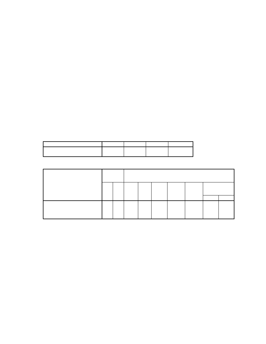
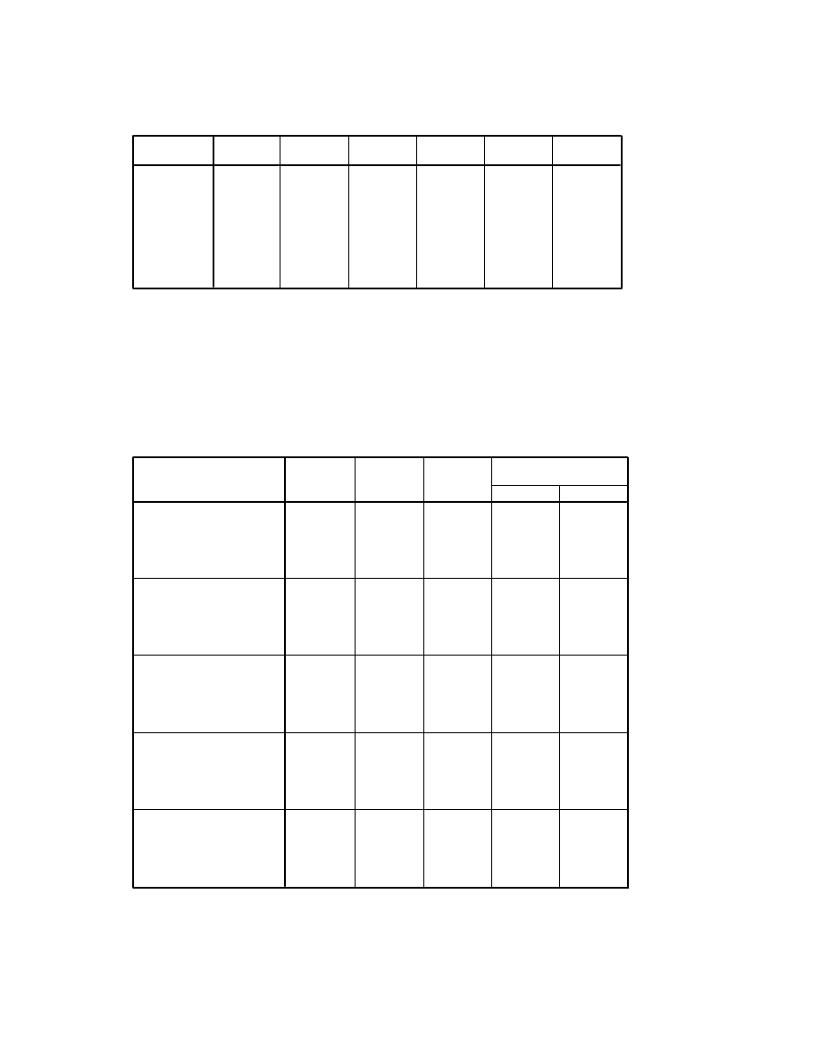
T-Test
Group Statistics
185
21.67
6.525
.480
251
22.90
6.911
.436
sex sex
MALES
FEMALES
tlifesat total life satisfaction
N
Mean
Std. Deviation
Std. Error Mean
Independent Samples Test
.706
.401
-1.881
434
.061
-1.230
.654
-2.516
.055
-1.897 408.528
.059
-1.230
.648
-2.505
.044
Equal variances
assumed
Equal variances not
assumed
tlifesat total
life satisfaction
F
Sig.
Levene's Test
for Equality of
Variances
t
df
Sig.
(2-tailed)
Mean
Difference
Std. Error
Difference
Lower
Upper
95% Confidence
Interval of the
Difference
t-test for Equality of Means
An independent-samples t-test was conducted to compare total life satisfaction scores for males
and females. There was no statistically significant difference between the two groups [t(434)
=-1.88, p=.06].
2
5.2 Using the data file experim.sav apply whichever of the t-test procedures covered in
Chapter 16 of the SPSS Survival Manual that you think are appropriate to answer the
following questions.
(a) Who has the greatest fear of statistics at time 1, males or females?
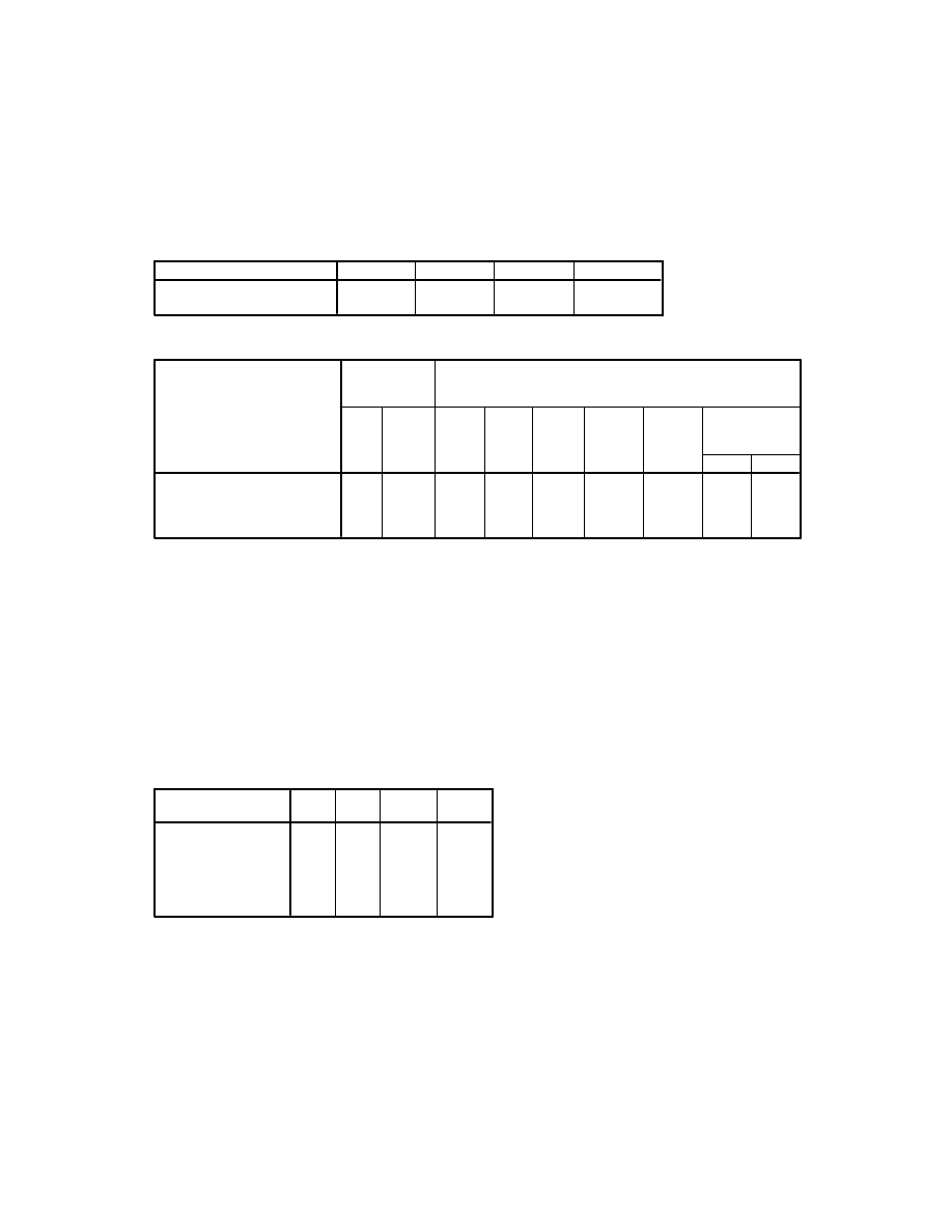
Group Statistics
15
41.20
5.685
1.468
15
39.13
4.533
1.171
sex
male
female
fost1 fear of stats time1
N
Mean
Std. Deviation
Std. Error Mean
Independent Samples Test
2.087
.160
1.101
28
.280
2.067
1.877
-1.779
5.912
1.101
26.679
.281
2.067
1.877
-1.788
5.921
Equal variances
assumed
Equal variances
not assumed
fost1 fear of
stats time1
F
Sig.
Levene's Test for
Equality of
Variances
t
df
Sig.
(2-tailed)
Mean
Difference
Std. Error
Difference
Lower
Upper
95% Confidence
Interval of the
Difference
t-test for Equality of Means
An independent-samples t-test was conducted to compare fear of statistics scores for males and
females. There was no statistically significant difference between the two groups [t(28) =1.10,
p=.28].
(b) Was the intervention effective in increasing students’ confidence in their ability to cope
with statistics? You will need to use the variables, confidence time1 (conf1) and confidence
time2 (conf2). Write your results up in a report.
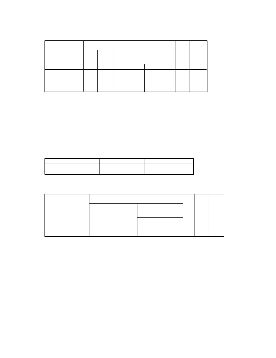
Paired Samples Statistics
19.00
30
5.369
.980
21.87
30
5.594
1.021
confid1
confidence
time1
confid2
confidence
time2
Pair 1
Mean
N
Std.
Deviation
Std. Error
Mean
3
Paired Samples Test
-2.867
4.754
.868
-4.642
-1.091
-3.303
29
.003
confid1
confidence
time1 - confid2
confidence
time2
Pair 1
Mean
Std.
Deviation
Std. Error
Mean
Lower
Upper
95% Confidence
Interval of the
Difference
Paired Differences
t
df
Sig.
(2-tailed)
A paired-samples t-test was conducted to assess whether there was a change in students’
confidence scores from time 1 (pre-intervention) to time 2 (post-intervention). There was a
statistically significant difference between the two sets of scores [t(29) =-3.30, p=.003]. Mean
scores increased from 19.0 (SD=5.37) at Time 1 to 21.87(SD=5.59) at Time 2.
(c) What impact did the intervention have on students’ levels of depression?
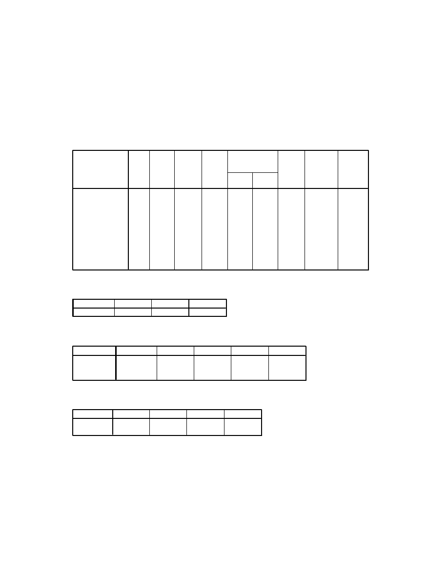
Paired Samples Statistics
42.53
30
4.592
.838
40.73
30
5.521
1.008
depress1 depression time1
depress2 depression time2
Pair 1
Mean
N
Std. Deviation
Std. Error Mean
Paired Samples Test
1.800
2.497
.456
.868
2.732
3.949
29
.000
depress1 depression
time1 - depress2
depression time2
Pair 1
Mean
Std.
Deviation
Std.
Error
Mean
Lower
Upper
95% Confidence Interval of
the Difference
Paired Differences
t
df
Sig.
(2-tailed)
A paired-samples t-test was conducted to assess whether there was a change in students’
depression scores from time 1 (pre-intervention) to time 2 (post-intervention). There was a
statistically significant difference between the two sets of scores [t(29) =-3.95, p<.001]. Mean
scores decreased from 42.53 (SD=4.59) at Time 1 to 40.73(SD=5.52) at Time 2.
4
One-way analysis of variance
For exercises 5.3 and 5.4 you will need to open the data file survey.sav.
5.3 Perform a one-way between-groups ANOVA to compare the levels of perceived stress
(tpstress) for the five different age groups (agegp5), 18-24yrs, 25-32yrs, 33-40yrs, 41-49yrs
and 50+yrs.
Descriptives
tpstress total perceived stress
93
28.60
6.094
.632
27.35
29.86
12
46
86
25.65
4.920
.531
24.60
26.71
14
39
82
26.77
5.918
.654
25.47
28.07
13
40
95
26.62
5.706
.585
25.46
27.78
12
42
77
25.75
6.178
.704
24.35
27.16
13
42
433
26.73
5.848
.281
26.18
27.28
12
46
5.774
.277
26.18
27.27
.539
25.23
28.22
1.062
18-24
25-32
33-40
41-49
50+
Total
Fixed
Effects
Random
Effects
Model
N
Mean
Std.
Deviation Std. Error
Lower
Bound
Upper
Bound
95% Confidence
Interval for Mean
Minimum
Maximum
Between-
Componen
t Variance
Test of Homogeneity of Variances
tpstress total perceived stress
1.340
4
428
.254
Levene Statistic
df1
df2
Sig.
ANOVA
tpstress total perceived stress
500.761
4
125.190
3.755
.005
14271.082
428
33.344
14771.843
432
Between Groups
Within Groups
Total
Sum of Squares
df
Mean Square
F
Sig.
Robust Tests of Equality of Means
tpstress total perceived stress
3.651
4
211.303
.007
3.744
4
411.700
.005
Welch
Brown-Forsythe
Statistic
a
df1
df2
Sig.
Asymptotically F distributed.
a.
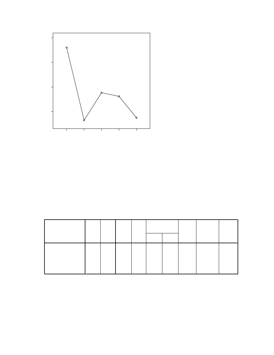
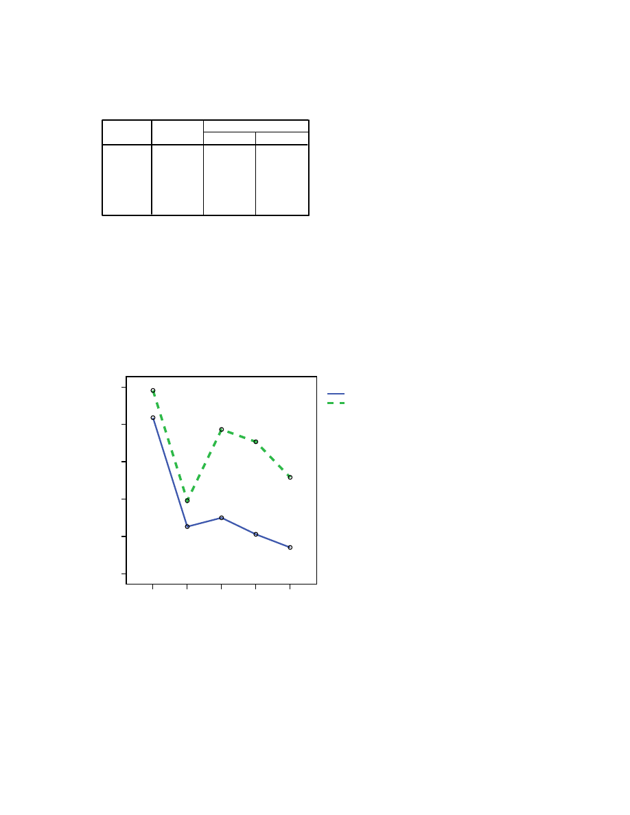
5
18-24
25-32
33-40
41-49
50+
age 5 groups
26
27
28
29
Mean of
tpstr
ess
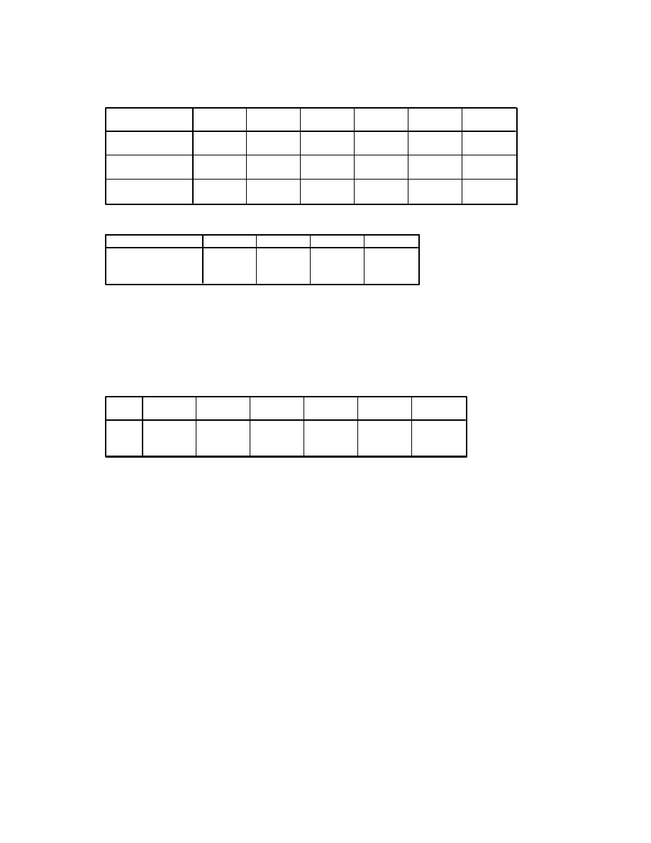
The results of the one way ANOVA indicate that there is a difference in the perceived stress
levels amongst the age groups [F(4, 428)=3.76, p=.005]. Inspection of the means plot
suggests that the younger age group (18 to 24yrs) has higher stress levels than the other age
groups.
5.4 Perform post-hoc tests to compare the Self esteem scores for people across the three
different age groups (use the agegp3 variable).
Descriptives
tslfest total self esteem
149
32.60
5.589
.458
31.69
33.50
18
40
152
33.59
5.288
.429
32.74
34.43
18
40
135
34.50
5.151
.443
33.63
35.38
20
40
436
33.53
5.395
.258
33.02
34.04
18
40
5.352
.256
33.03
34.04
.545
31.19
35.88
.692
18-29
30-44
45+
Total
Fixed Effects
Random Effects
Model
N
Mean
Std.
Deviation
Std.
Error
Lower
Bound
Upper
Bound
95% Confidence
Interval for Mean
Minimum
Maximum
Between-
Componen
t Variance

6
tslfest total self esteem
149
32.60
152
33.59
33.59
135
34.50
.259
.311
149
32.60
152
33.59
33.59
135
34.50
agegp3 age 3 groups
18-29
30-44
45+
Sig.
18-29
30-44
45+
Sig.
Tukey HSD
a,b
Tukey B
a,b
N
1
2
Subset for alpha = .05
Means for groups in homogeneous subsets are displayed.
Uses Harmonic Mean Sample Size = 144.943.
a.
The group sizes are unequal. The harmonic mean of the group sizes is
used. Type I error levels are not guaranteed.
b.
Post-hoc comparisons using the Tukey Honestly Significant Difference test indicated that the
mean score for Group 1 (M=32.6, SD=5.59) was significantly different from Group 3 (M=34.5,
SD=5.15). Group 2 (M=33.59, SD=5.29) did not differ significantly from either Group 1 or 3.
For the following exercise you will need to open the data file experim.sav.
5.5 Use one-way repeated measures ANOVA to compare the Fear of Statistics scores for the
three time periods (time1, time2 and time3). Inspect the means plots and describe the impact
of the intervention and the subsequent follow-up three months later.
General Linear Model
Within-Subjects Factors
Measure: MEASURE_1
fost1
fost2
fost3
time
1
2
3
Dependent
Variable
Descriptive Statistics
40.17
5.160
30
37.50
5.151
30
35.23
6.015
30
fost1 fear of stats time1
fost2 fear of stats time2
fost3 fear of stats time3
Mean
Std. Deviation
N
7
Multivariate Tests
b
.635
24.356
a
2.000
28.000
.000
.635
.365
24.356
a
2.000
28.000
.000
.635
1.740
24.356
a
2.000
28.000
.000
.635
1.740
24.356
a
2.000
28.000
.000
.635
Pillai's Trace
Wilks' Lambda
Hotelling's Trace
Roy's Largest Root
Effect
time
Value
F
Hypothesis df
Error df
Sig.
Partial Eta
Squared
Exact statistic
a.
Design: Intercept
Within Subjects Design: time
b.
Mauchly's Test of Sphericity
b
Measure: MEASURE_1
.342
30.071
2
.000
.603
.615
.500
Within Subjects Effect
time
Mauchly's W
Approx.
Chi-Square
df
Sig.
Greenhouse-
Geisser
Huynh-Feldt
Lower-bound
Epsilon
a
Tests the null hypothesis that the error covariance matrix of the orthonormalized transformed dependent variables is proportional to an
identity matrix.
May be used to adjust the degrees of freedom for the averaged tests of significance. Corrected tests are displayed in the
Tests of Within-Subjects Effects table.
a.
Design: Intercept
Within Subjects Design: time
b.
Tests of Within-Subjects Effects
Measure: MEASURE_1
365.867
2
182.933
41.424
.000
.588
365.867
1.206
303.368
41.424
.000
.588
365.867
1.230
297.506
41.424
.000
.588
365.867
1.000
365.867
41.424
.000
.588
256.133
58
4.416
256.133
34.974
7.323
256.133
35.664
7.182
256.133
29.000
8.832
Sphericity Assumed
Greenhouse-Geisser
Huynh-Feldt
Lower-bound
Sphericity Assumed
Greenhouse-Geisser
Huynh-Feldt
Lower-bound
Source
time
Error(time)
Type III Sum
of Squares
df
Mean Square
F
Sig.
Partial Eta
Squared
Tests of Within-Subjects Contrasts
Measure: MEASURE_1
365.067
1
365.067
46.652
.000
.617
.800
1
.800
.795
.380
.027
226.933
29
7.825
29.200
29
1.007
time
Linear
Quadratic
Linear
Quadratic
Source
time
Error(time)
Type III Sum
of Squares
df
Mean Square
F
Sig.
Partial Eta
Squared
8
Tests of Between-Subjects Effects
Measure: MEASURE_1
Transformed Variable: Average
127464.100
1
127464.100
1583.134
.000
.982
2334.900
29
80.514
Source
Intercept
Error
Type III Sum
of Squares
df
Mean Square
F
Sig.
Partial Eta
Squared
1
2
3
time
35
36
37
38
39
40
41
E
sti
m
ate
d
M
arg
ina
l Me
a
n
s
Estimated Marginal Means of MEASURE_1
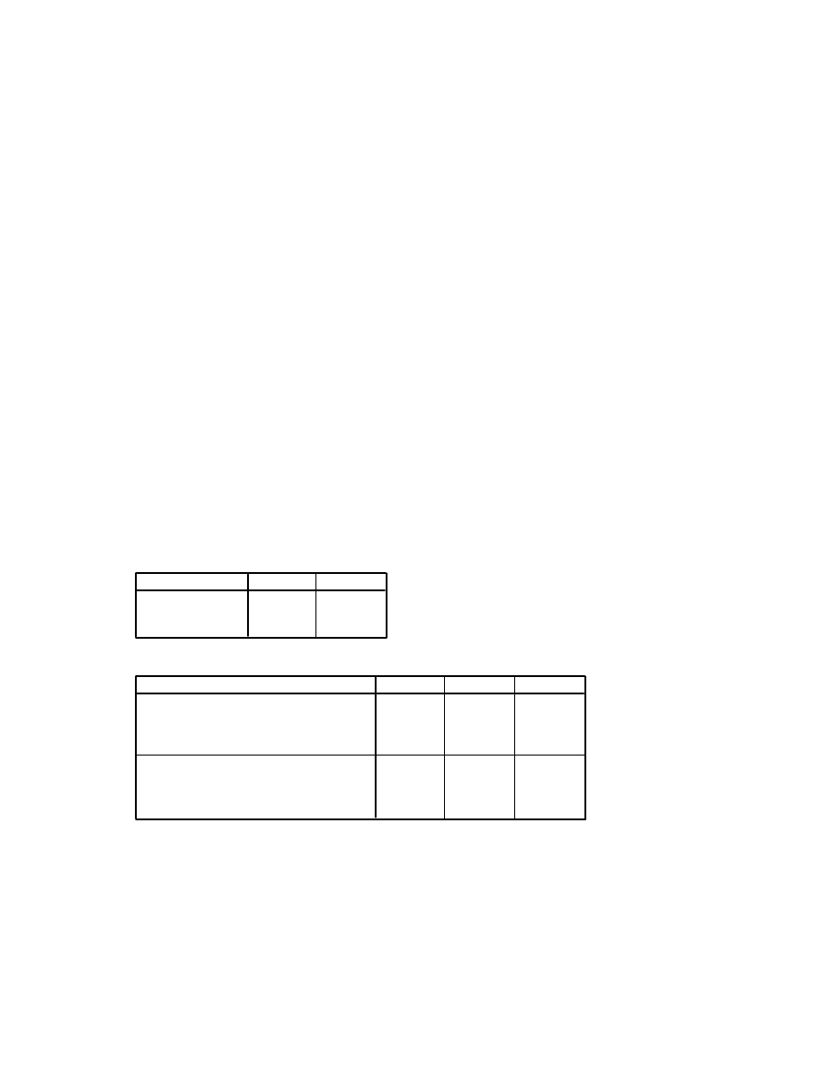
A one way repeated measures ANOVA was conducted to compare scores on the Fear of
Statistics Test scores at Time 1(prior to the intervention), Time 2 (following the intervention)
and Time 3 (three month follow-up). There was a significant effect for time [Wilks’ Lambda=
.365, F(2,28 )=24.36, p<.0005, multivariate partial eta squared=.64. Inspection of the plot of
mean values indicate a steady decrease in fear scores following the intervention, and at the
three month follow-up.
9
Two-way between-groups ANOVA
5.6 For this exercise you will need to open the data file survey.sav. Follow the instructions in
Chapter 18 of the SPSS Survival Manual to conduct a two-way ANOVA to explore the impact
of sex and age group on levels of perceived stress. The three variables you will need are sex,
agegp5 and tpstress.
(a) Interpret the results. Is there a significant interaction effect? Are the two main effects
significant?
Univariate Analysis of Variance
Between-Subjects Factors
MALES
184
FEMALES
249
18-24
93
25-32
86
33-40
82
41-49
95
50+
77
1
2
sex sex
1
2
3
4
5
agegp5
age 5
groups
Value Label
N
Descriptive Statistics
Dependent Variable: tpstress total perceived stress
28.18
5.619
39
25.26
4.774
38
25.50
5.177
38
25.06
4.802
35
24.71
6.157
34
25.79
5.414
184
28.91
6.449
54
25.96
5.061
48
27.86
6.345
44
27.53
6.024
60
26.58
6.138
43
27.42
6.066
249
28.60
6.094
93
25.65
4.920
86
26.77
5.918
82
26.62
5.706
95
25.75
6.178
77
26.73
5.848
433
agegp5 age 5 groups
18-24
25-32
33-40
41-49
50+
Total
18-24
25-32
33-40
41-49
50+
Total
18-24
25-32
33-40
41-49
50+
Total
sex sex
MALES
FEMALES
Total
Mean
Std. Deviation
N
Levene's Test of Equality of Error Variances
a
Dependent Variable: tpstress total perceived stress
1.026
9
423
.418
F
df1
df2
Sig.
Tests the null hypothesis that the error variance of the
dependent variable is equal across groups.
Design: Intercept+sex+agegp5+sex * agegp5
a.
10
Tests of Between-Subjects Effects
Dependent Variable: tpstress total perceived stress
839.252
a
9
93.250
2.831
.003
.057
295968.489
1
295968.489
8985.743
.000
.955
277.994
1
277.994
8.440
.004
.020
503.367
4
125.842
3.821
.005
.035
64.874
4
16.219
.492
.741
.005
13932.591
423
32.938
324089.000
433
14771.843
432
Source
Corrected Model
Intercept
sex
agegp5
sex * agegp5
Error
Total
Corrected Total
Type III Sum
of Squares
df
Mean Square
F
Sig.
Partial Eta
Squared
R Squared = .057 (Adjusted R Squared = .037)
a.
Post Hoc Tests
agegp5 age 5 groups
Multiple Comparisons
Dependent Variable: tpstress total perceived stress
Tukey HSD
2.95*
.859
.006
.60
5.30
1.83
.869
.218
-.55
4.22
1.98
.837
.127
-.31
4.27
2.85*
.884
.012
.43
5.27
-2.95*
.859
.006
-5.30
-.60
-1.12
.886
.715
-3.54
1.31
-.97
.854
.788
-3.31
1.37
-.10
.900
1.000
-2.57
2.36
-1.83
.869
.218
-4.22
.55
1.12
.886
.715
-1.31
3.54
.15
.865
1.000
-2.22
2.52
1.02
.911
.799
-1.48
3.51
-1.98
.837
.127
-4.27
.31
.97
.854
.788
-1.37
3.31
-.15
.865
1.000
-2.52
2.22
.87
.880
.862
-1.54
3.28
-2.85*
.884
.012
-5.27
-.43
.10
.900
1.000
-2.36
2.57
-1.02
.911
.799
-3.51
1.48
-.87
.880
.862
-3.28
1.54
(J) age 5 groups
18-24
25-32
33-40
41-49
50+
18-24
25-32
33-40
41-49
50+
18-24
25-32
33-40
41-49
50+
18-24
25-32
33-40
41-49
50+
18-24
25-32
33-40
41-49
50+
(I) age 5 groups
18-24
25-32
33-40
41-49
50+
Mean
Difference (I-J)
Std. Error
Sig.
Lower Bound
Upper Bound
95% Confidence Interval
Based on observed means.
The mean difference is significant at the .05 level.
*.
11
Homogeneous Subsets
tpstress total perceived stress
Tukey HSD
a,b,c
86
25.65
77
25.75
95
26.62
26.62
82
26.77
26.77
93
28.60
.706
.159
age 5 groups
25-32
50+
41-49
33-40
18-24
Sig.
N
1
2
Subset
Means for groups in homogeneous subsets are displayed.
Based on Type III Sum of Squares
The error term is Mean Square(Error) = 32.938.
Uses Harmonic Mean Sample Size = 86.075.
a.
The group sizes are unequal. The harmonic mean of the
group sizes is used. Type I error levels are not guaranteed.
b.
Alpha = .05.
c.
18-24
25-32
33-40
41-49
50+
age 5 groups
24
25
26
27
28
29
Estim
ated M
arginal Means
sex
MALES
FEMALES
Estimated Marginal Means of total perceived stress
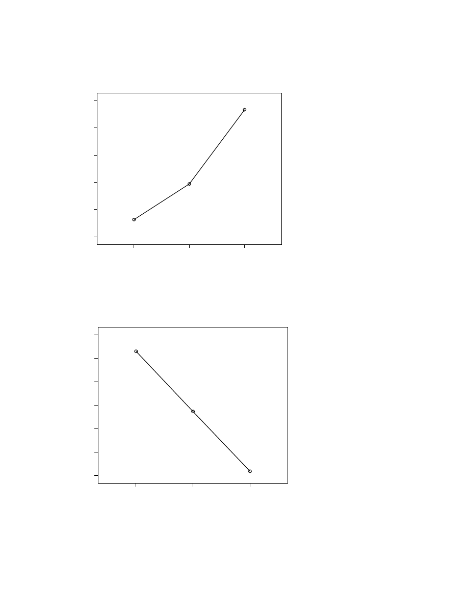
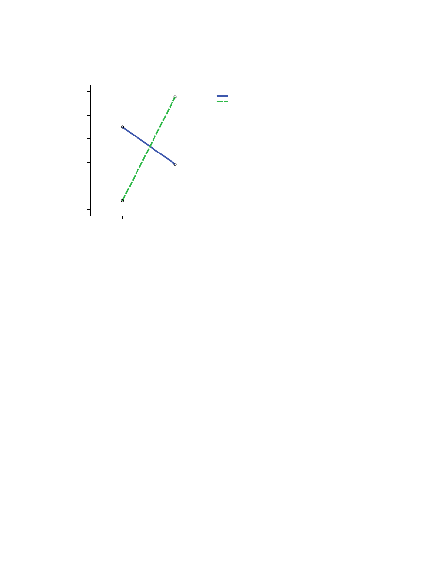
The interaction effect (sex*agegp5) did not reach statistical significance[F(4, 423)=.492,
p=.741), however there was a significant main effect for sex [F(1,423)=8.44,p=.004) and age
group [F(4,423)=3.82, p=.005). Inspection of the mean scores and the plot suggest that
overall males have lower levels of perceived stress at all age levels. Overall younger people
(18 to 24 yrs) reported higher levels of stress than the other age groups. The results of this
analysis shows that although the means plot suggests the possibility of an interaction between
age and gender, it did not reach statistical significance.

12
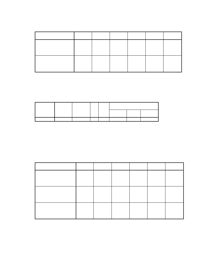
(b) Write up this analysis and the results in a report. (Don’t forget to report the means and
standard deviations for each group.)
A two-way between groups analysis of variance was conducted to explore the impact of sex
and age on levels of perceived stress, as measured by the Perceived Stress Scale. Subjects
were divided into five groups according to their age (Group 1: 18 to 24years; Group 2: 25 to
32yrs; Group 3: 33 to 40yrs; Group 4: 41 to 49yrs; Group 5: 50yrs and above). There was no
significant interaction effect between age and sex [F(4,423)=.49, p=.74]. The main effect for
both sex [F(1,423)=8.44, p=.004, partial eta squared=.02] and age [F(4,423)=3.82, p=.005,
partial eta squared=.035] was statistically significant. Post hoc tests using Tukey’s Honestly
Significance Difference test revealed that the 18 to 24yr age group differed significantly from
the 25 to 32yr age group and the 50+ age group. All other group comparisons did not reach
statistical significance. Table XX below shows the mean scores for males and females for
each of the age groups.
Table XX
Mean and Standard Deviations for Males and Females across Age Groups
Males
Females
n
Mean
SD n
Mean SD
18-24yrs 39 28.18 5.62
54 28.91
6.45
25-32yrs 38 25.26 4.77
48 25.96
5.06
33-40yrs 38 25.50 5.18
44 27.86
6.35
41-49yrs 35 25.06 6.16
60 27.53
6.02
50+ 34
24.70 6.16 43 26.58 6.14
13
Mixed between-within subjects analysis of variance
5.7 In Chapter 19 of the SPSS Survival Manual we explored the impact of two different
intervention programs (maths skills/confidence building) on participants’ fear of statistics. We
found that both interventions were equally effective in reducing participants’ fear—that is, we
found no differences between groups—but a significant difference across the three time
periods. Repeat these analyses, but this time use confidence scores as the dependent variable.
Open the file experim.sav. You will need to use the following variables: group, conf1, conf2
and conf3.
General Linear Model
Within-Subjects Factors
Measure: MEASURE_1
confid1
confid2
confid3
time
1
2
3
Dependent
Variable
Between-Subjects Factors
maths skills
15
confidence
building
15
1
2
group type
of class
Value Label
N
Descriptive Statistics
18.87
5.527
15
19.13
5.397
15
19.00
5.369
30
20.00
4.660
15
23.73
5.970
15
21.87
5.594
30
24.07
4.543
15
26.00
5.782
15
25.03
5.203
30
group type of class
maths skills
confidence building
Total
maths skills
confidence building
Total
maths skills
confidence building
Total
confid1 confidence time1
confid2 confidence time2
confid3 confidence time3
Mean
Std. Deviation
N
Box's Test of Equality of Covariance Matrices
a
8.522
1.254
6
5680.302
.275
Box's M
F
df1
df2
Sig.
Tests the null hypothesis that the observed covariance
matrices of the dependent variables are equal across groups.
Design: Intercept+group
Within Subjects Design: time
a.
14
Multivariate Tests
b
.752
40.897
a
2.000
27.000
.000
.752
.248
40.897
a
2.000
27.000
.000
.752
3.029
40.897
a
2.000
27.000
.000
.752
3.029
40.897
a
2.000
27.000
.000
.752
.207
3.534
a
2.000
27.000
.043
.207
.793
3.534
a
2.000
27.000
.043
.207
.262
3.534
a
2.000
27.000
.043
.207
.262
3.534
a
2.000
27.000
.043
.207
Pillai's Trace
Wilks' Lambda
Hotelling's Trace
Roy's Largest Root
Pillai's Trace
Wilks' Lambda
Hotelling's Trace
Roy's Largest Root
Effect
time
time * group
Value
F
Hypothesis df
Error df
Sig.
Partial Eta
Squared
Exact statistic
a.
Design: Intercept+group
Within Subjects Design: time
b.
Mauchly's Test of Sphericity
b
Measure: MEASURE_1
.573
15.059
2
.001
.701
.753
.500
Within
Subjects Effect
time
Mauchly's W
Approx.
Chi-Square
df
Sig.
Greenhouse-
Geisser
Huynh-
Feldt
Lower-bound
Epsilon
a
Tests the null hypothesis that the error covariance matrix of the orthonormalized transformed dependent
variables is proportional to an identity matrix.
May be used to adjust the degrees of freedom for the averaged tests of significance. Corrected
tests are displayed in the Tests of Within-Subjects Effects table.
a.
Design: Intercept+group
Within Subjects Design: time
b.
Tests of Within-Subjects Effects
Measure: MEASURE_1
546.467
2
273.233
35.383
.000
.558
546.467
1.401
390.038
35.383
.000
.558
546.467
1.505
363.097
35.383
.000
.558
546.467
1.000
546.467
35.383
.000
.558
45.089
2
22.544
2.919
.062
.094
45.089
1.401
32.182
2.919
.082
.094
45.089
1.505
29.959
2.919
.079
.094
45.089
1.000
45.089
2.919
.099
.094
432.444
56
7.722
432.444
39.230
11.023
432.444
42.140
10.262
432.444
28.000
15.444
Sphericity Assumed
Greenhouse-Geisser
Huynh-Feldt
Lower-bound
Sphericity Assumed
Greenhouse-Geisser
Huynh-Feldt
Lower-bound
Sphericity Assumed
Greenhouse-Geisser
Huynh-Feldt
Lower-bound
Source
time
time * group
Error(time)
Type III Sum
of Squares
df
Mean Square
F
Sig.
Partial Eta
Squared
15
Tests of Within-Subjects Contrasts
Measure: MEASURE_1
546.017
1
546.017
52.526
.000
.652
.450
1
.450
.089
.767
.003
10.417
1
10.417
1.002
.325
.035
34.672
1
34.672
6.867
.014
.197
291.067
28
10.395
141.378
28
5.049
time
Linear
Quadratic
Linear
Quadratic
Linear
Quadratic
Source
time
time * group
Error(time)
Type III Sum
of Squares
df
Mean Square
F
Sig.
Partial Eta
Squared
Levene's Test of Equality of Error Variances
a
.000
1
28
.986
1.718
1
28
.201
.873
1
28
.358
confid1 confidence time1
confid2 confidence time2
confid3 confidence time3
F
df1
df2
Sig.
Tests the null hypothesis that the error variance of the dependent variable is equal
across groups.
Design: Intercept+group
Within Subjects Design: time
a.
Tests of Between-Subjects Effects
Measure: MEASURE_1
Transformed Variable: Average
43428.100
1
43428.100
619.488
.000
.957
88.011
1
88.011
1.255
.272
.043
1962.889
28
70.103
Source
Intercept
group
Error
Type III Sum
of Squares
df
Mean Square
F
Sig.
Partial Eta
Squared

16
1
2
3
time
18
20
22
24
26
Estimated Marginal Means
type of class
maths skills
confidence
building
Estimated Marginal Means of MEASURE_1
(a) Is there a significant interaction effect between type of intervention (group) and time?
The interaction between type of intervention and time is significant (p=.043). An inspection of
the plot suggests that the confidence building group showed greater improvement in
confidence levels following the intervention than the maths skills group.
(b) Is there a significant main effect for the within-subjects independent variable, time?
The interaction effect for group by time is significant, therefore it is not really appropriate to
interpret the main effect. The impact of one variable (eg. Time) is dependent on the level of
the other variable (group).
(c) Is there a significant main effect for the between-subjects independent variable, group
(maths skills/confidence building)?
The interaction effect for group by time is significant, therefore it is not appropriate to
interpret the main effect. The impact of one variable (eg. Time) is dependent on the level of
the other variable (group).
17
Multivariate analysis of variance
5.8 How does MANOVA differ from ANOVA?
Multivariate analysis of variance is an extension of analysis of variance for use when there is
more than one dependent variable.
5.9 In Chapter 20 of the SPSS Survival Manual it is recommended that you check the
Mahalonobis distances before proceeding with MANOVA. What does this allow you to check
for?
Mahalonobis distances is a test of multivariate normality.
5.10 Which assumption is Box’s M Test used to assess?
Box’s M Test is used to assess the homogeneity of variance-covariance matrices.
5.11 Follow the procedure detailed in Chapter 20 of the SPSS Survival Manual to perform a
MANOVA to explore positive and negative affect scores for the three age groups (18-29yrs,
30-44yrs, 45+yrs). The three variables you will need are tposaff, tnegaff, agegp3. Remember
to check your assumptions.
General Linear Model
Between-Subjects Factors
18-29
147
30-44
153
45+
135
1
2
3
agegp3 age
3 groups
Value Label
N
Descriptive Statistics
33.33
7.409
147
33.59
7.316
153
34.13
7.017
135
33.67
7.247
435
20.65
7.346
147
19.37
6.616
153
18.09
7.076
135
19.40
7.072
435
agegp3 age 3 groups
18-29
30-44
45+
Total
18-29
30-44
45+
Total
tposaff total positive affect
tnegaff total negative affect
Mean
Std. Deviation
N

18
Box's Test of Equality of Covariance Matrices
a
2.703
.448
6
4335850.466
.847
Box's M
F
df1
df2
Sig.
Tests the null hypothesis that the observed covariance
matrices of the dependent variables are equal across groups.
Design: Intercept+agegp3
a.
Multivariate Tests
c
.976
8661.453
a
2.000
431.000
.000
.976
.024
8661.453
a
2.000
431.000
.000
.976
40.192
8661.453
a
2.000
431.000
.000
.976
40.192
8661.453
a
2.000
431.000
.000
.976
.021
2.340
4.000
864.000
.054
.011
.979
2.347
a
4.000
862.000
.053
.011
.022
2.354
4.000
860.000
.052
.011
.022
4.709
b
2.000
432.000
.009
.021
Pillai's Trace
Wilks' Lambda
Hotelling's Trace
Roy's Largest Root
Pillai's Trace
Wilks' Lambda
Hotelling's Trace
Roy's Largest Root
Effect
Intercept
agegp3
Value
F
Hypothesis df
Error df
Sig.
Partial Eta
Squared
Exact statistic
a.
The statistic is an upper bound on F that yields a lower bound on the significance level.
b.
Design: Intercept+agegp3
c.
Levene's Test of Equality of Error Variances
a
.350
2
432
.705
.970
2
432
.380
tposaff total positive affect
tnegaff total negative affect
F
df1
df2
Sig.
Tests the null hypothesis that the error variance of the dependent variable is equal across
groups.
Design: Intercept+agegp3
a.
Tests of Between-Subjects Effects
47.346
a
2
23.673
.450
.638
.002
463.048
b
2
231.524
4.709
.009
.021
492175.882
1
492175.882
9347.172
.000
.956
162755.374
1
162755.374
3310.007
.000
.885
47.346
2
23.673
.450
.638
.002
463.048
2
231.524
4.709
.009
.021
22746.985
432
52.655
21241.743
432
49.171
515910.000
435
185499.000
435
22794.331
434
21704.791
434
Dependent Variable
tposaff total positive affect
tnegaff total negative affect
tposaff total positive affect
tnegaff total negative affect
tposaff total positive affect
tnegaff total negative affect
tposaff total positive affect
tnegaff total negative affect
tposaff total positive affect
tnegaff total negative affect
tposaff total positive affect
tnegaff total negative affect
Source
Corrected Model
Intercept
agegp3
Error
Total
Corrected Total
Type III Sum
of Squares
df
Mean Square
F
Sig.
Partial Eta
Squared
R Squared = .002 (Adjusted R Squared = -.003)
a.
R Squared = .021 (Adjusted R Squared = .017)
b.
19
18-29
30-44
45+
age 3 groups
33.2
33.4
33.6
33.8
34
34.2
Estimate
d Mar
g
inal M
e
ans
Estimated Marginal Means of total positive affect
18-29
30-44
45+
age 3 groups
18
18.5
19
19.5
20
20.5
21
Estimated
Marg
in
al
Means
Estimated Marginal Means of total negative affect

20
The results of Box’s test of equality of covariance matrices indicate no violation of the
assumption (p=.85)
The results of Levene’s test of equality of error variances indicate that we have not violated
the assumption for either of our dependent variables (p=.71, p=.38).
Inspection of the results shown in Multivariate tests indicate a significant result overall
[Wilks’ Lambda=.98, F(4, 862)=2.35, p=.05].
The Tests of Between Subjects Effects table indicates a significant result for Total Negative
Affect [F(2,432)=4.71, p=.009, partial eta squared=.02], but not for Total Positive Affect
[F(2,432)=.45, p=.64, partial eta squared=.002]. Inspection of the mean scores for each age
group indicates a steady decrease in levels of negative affect across the three age groups (18-
29yrs mean=20.65, SD=7.35; 30-44yrs mean=19.37, SD=6.62; 45+yrs mean=18.09,
SD=7.07).
21
Analysis of covariance
5.12 Under what circumstances would you want to consider using analysis of covariance?
Analysis of covariance is used when you wish to compare groups, while controlling for
additional variables that you suspect might be influencing scores on the dependent variable.
5.13 What issues do you need to consider when you are selecting possible covariates?
Covariates need to be chosen with a good understanding of background theory and previous
research in your research area. The covariates need to be continuous variables, measured
reliably and correlate significantly with the dependent variable. The covariate must be
measured before the treatment or experimental manipulation is conducted.
5.14 Using the experim.sav data file, perform the appropriate analyses (including assumption
testing) to compare the confidence scores for the two groups (maths skills, confidence
building) at time 2, while controlling for confidence scores at time 1. The variables you will
need are group, conf1, conf2.
Univariate Analysis of Variance
Between-Subjects Factors
maths skills
15
confidence
building
15
1
2
group type
of class
Value Label
N
Tests of Between-Subjects Effects
Dependent Variable: confid2 confidence time2
466.737
a
3
155.579
9.178
.000
196.989
1
196.989
11.621
.002
2.067
1
2.067
.122
.730
348.104
1
348.104
20.536
.000
17.644
1
17.644
1.041
.317
440.730
26
16.951
15252.000
30
907.467
29
Source
Corrected Model
Intercept
group
confid1
group * confid1
Error
Total
Corrected Total
Type III Sum
of Squares
df
Mean Square
F
Sig.
R Squared = .514 (Adjusted R Squared = .458)
a.
The above output is used to assess the assumption of homogeneity of regression slopes. The
interaction term (group*confid1) is not significant (p=.317), therefore we have not violated
the assumption and can then proceed with the ANCOVA analysis.
22
Univariate Analysis of Variance
Between-Subjects Factors
maths skills
15
confidence
building
15
1
2
group type
of class
Value Label
N
Descriptive Statistics
Dependent Variable: confid2 confidence time2
20.00
4.660
15
23.73
5.970
15
21.87
5.594
30
group type of class
maths skills
confidence building
Total
Mean
Std. Deviation
N
Levene's Test of Equality of Error Variances
a
Dependent Variable: confid2 confidence time2
.136
1
28
.715
F
df1
df2
Sig.
Tests the null hypothesis that the error variance of the
dependent variable is equal across groups.
Design: Intercept+confid1+group
a.
Tests of Between-Subjects Effects
Dependent Variable: confid2 confidence time2
449.093
a
2
224.546
13.227
.000
.495
200.700
1
200.700
11.822
.002
.305
344.560
1
344.560
20.296
.000
.429
95.102
1
95.102
5.602
.025
.172
458.374
27
16.977
15252.000
30
907.467
29
Source
Corrected Model
Intercept
confid1
group
Error
Total
Corrected Total
Type III Sum
of Squares
df
Mean Square
F
Sig.
Partial Eta
Squared
R Squared = .495 (Adjusted R Squared = .457)
a.
Estimated Marginal Means
type of class
Dependent Variable: confid2 confidence time2
20.086
a
1.064
17.902
22.269
23.648
a
1.064
21.465
25.831
type of class
maths skills
confidence building
Mean
Std. Error
Lower Bound
Upper Bound
95% Confidence Interval
Covariates appearing in the model are evaluated at the following
values: confid1 confidence time1 = 19.00.
a.

23
Inspection of the table ‘Levene’s Test of Equality of Error Variances’ indicate we have not
violated the assumption concerning the equality of variances (p=.715).
The Tests of Between-Subjects Effects table results indicate a significant effect for group
(p=.025). There is a significant difference in confidence scores for the confidence building
and maths skills groups, after controlling for confidence scores administered prior to the
treatment program.
5.15 Perform a two-way analysis of covariance to explore the question: Does gender influence
the effectiveness of the two intervention programs designed to increase participants’
confidence in being able to cope with statistics training? You will need to assess the impact of
sex and type of intervention (group) on confidence at time 2, controlling for confidence scores
at time 1.
Univariate Analysis of Variance
Between-Subjects Factors
maths skills
15
confidence
building
15
male
15
female
15
1
2
group type
of class
1
2
sex
Value Label
N
Descriptive Statistics
Dependent Variable: confid2 confidence time2
22.25
4.301
8
17.43
3.823
7
20.00
4.660
15
21.29
5.880
7
25.88
5.515
8
23.73
5.970
15
21.80
4.931
15
21.93
6.364
15
21.87
5.594
30
sex
male
female
Total
male
female
Total
male
female
Total
group type of class
maths skills
confidence building
Total
Mean
Std. Deviation
N
Levene's Test of Equality of Error Variances
a
Dependent Variable: confid2 confidence time2
2.277
3
26
.103
F
df1
df2
Sig.
Tests the null hypothesis that the error variance of the
dependent variable is equal across groups.
Design: Intercept+confid1+group+sex+group * sex
a.
24
Tests of Between-Subjects Effects
Dependent Variable: confid2 confidence time2
826.891
a
4
206.723
64.139
.000
.911
55.142
1
55.142
17.109
.000
.406
556.942
1
556.942
172.800
.000
.874
92.813
1
92.813
28.797
.000
.535
.815
1
.815
.253
.620
.010
377.226
1
377.226
117.040
.000
.824
80.576
25
3.223
15252.000
30
907.467
29
Source
Corrected Model
Intercept
confid1
group
sex
group * sex
Error
Total
Corrected Total
Type III Sum
of Squares
df
Mean Square
F
Sig.
Partial Eta
Squared
R Squared = .911 (Adjusted R Squared = .897)
a.
Estimated Marginal Means
1. type of class
Dependent Variable: confid2 confidence time2
19.855
a
.465
18.898
20.811
23.381
a
.465
22.424
24.339
type of class
maths skills
confidence building
Mean
Std. Error
Lower Bound
Upper Bound
95% Confidence Interval
Covariates appearing in the model are evaluated at the following
values: confid1 confidence time1 = 19.00.
a.
2. sex
Dependent Variable: confid2 confidence time2
21.783
a
.465
20.826
22.740
21.453
a
.465
20.495
22.410
sex
male
female
Mean
Std. Error
Lower Bound
Upper Bound
95% Confidence Interval
Covariates appearing in the model are evaluated at the
following values: confid1 confidence time1 = 19.00.
a.
3. type of class * sex
Dependent Variable: confid2 confidence time2
23.750
a
.645
22.422
25.078
15.959
a
.688
14.543
17.375
19.816
a
.688
18.400
21.232
26.947
a
.640
25.629
28.265
sex
male
female
male
female
type of class
maths skills
confidence building
Mean
Std. Error
Lower Bound
Upper Bound
95% Confidence Interval
Covariates appearing in the model are evaluated at the following values: confid1
confidence time1 = 19.00.
a.
25
maths skills
confidence building
type of class
15
17.5
20
22.5
25
27.5
Es
ti
ma
te
d Ma
rg
in
al
M
ea
n
s
sex
male
female
Estimated Marginal Means of confidence time2
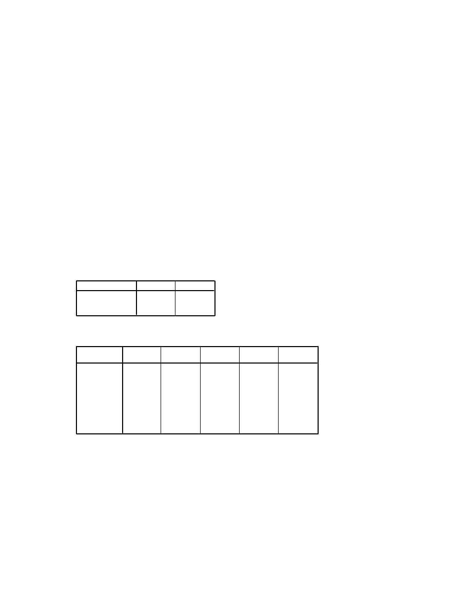
An inspection of the plot of mean scores suggests the possibility of an interaction between
gender and type of intervention in terms of confidence scores. Females in the Confidence
building group showed higher confidence scores at Time 2, than those who received the
Maths skills intervention. Males however who participated in the Maths skills intervention
showed higher mean scores than those who were in the Confidence Building group. This is
supported by the results in the Tests of Between Subjects Effects table. The group*sex
interaction term is statistically significant [F(1,25)=117.04, p<.0005].

26
Non-parametric statistics
5.16 What is the difference between parametric techniques and non-parametric techniques?
The parametric tests (eg. T-tests, ANOVA) make assumptions about the population the sample
has been drawn from. Non-parametric techniques do not have such stringent requirements
and do not make assumptions about the underlying population distribution.
5.17 What factors would you consider when choosing whether to use a parametric or a non-
parametric technique?
You need to consider the levels of measurement of your data. If you have nominal or ordinal
scaled data you should use a suitable non-parametric, rather than parametric technique.
5.18 For each of the following parametric techniques indicate the non-parametric alternative
(if one exists).
(a) one-way between-groups ANOVA
Kruskal-Wallis Test
(b) Pearson’s product-moment correlation
Spearman Rank Order Correlation
(c) independent samples t-test
Mann-Whitney Test
(d) multivariate analysis of variance
No equivalent
(e) one-way repeated measures ANOVA
Friedman Test
(f) paired samples t-test
Wilcoxon Signed Rank Test
(g) partial correlation
No equivalent
5.19 Choose and perform the appropriate non-parametric test to address each of the following
research questions.
(a) Using the survey.sav data file find out whether smokers are significantly more stressed
than non-smokers. The variables you will need are smoke and total perceived stress (tpstress).
Mann-Whitney Test
(b) Using the survey.sav data file compare the self-esteem scores across the three different age
groups (18-29yrs, 30-44yrs, 45+yrs). The variables you will need are tslfest and agegp3.
Kruskal-Wallis Test.
(c) Using the survey.sav data file explore the relationship between optimism and negative
affect. The variables you will need are toptim and tnegaff.
Spearman Rank Order Correlation
(d) Using the survey.sav data file explore the association between education level and
smoking. The variables you will need are educ2 and smoke. Check the codebook and the
questionnaire in the appendix of the SPSS Survival Manual for details on these two variables.
Chi square test for independence

27
(e) Using the experim.sav data file compare the depression scores at time 1 and the depression
scores at time 2. Did the intervention result in a significant change in depression scores? The
variables you will need are depress1 and depress2.
Wilcoxon Signed Rank Test
(f) Using the experim.sav data file compare the depression scores for the three time periods
involved in the study (before the intervention, after the intervention and at the three-month
follow up). The variables you will need are depress1, depress2 and depress3.
Friedman Test
Wyszukiwarka
Podobne podstrony:
08 COMPARE GROUPS
eim2 09 answers
eim3 09 answer
semquiz 09-5 answers, 1
25)21 09 To? questions and short answers Va
semquiz 09-4 answers, 1
22)20 09 Present continuous questions and answers IVa
eim2 09 answers
eim3 09 answer
grammar games comparatives and superlatives answers
EF3e int filetest 09 answerkey
download Zarządzanie Produkcja Archiwum w 09 pomiar pracy [ www potrzebujegotowki pl ]
09 AIDSid 7746 ppt
09 Architektura systemow rozproszonychid 8084 ppt
TOiZ 09
comparative superlative
Wyklad 2 TM 07 03 09
więcej podobnych podstron