MODELLING OF VOLATILE ORGANIC COMPOUNDS EMISSION FROM

DRY BUILDING MATERIALS

Hongyu Huang

Fariborz Haghighat

Department of Building, Civil and Environmental Engineering

Concordia University, Montreal, Canada

hongyu_h@ cbs-engr.concordia.ca

haghi@ cbs-engr.concordia.ca

ABSTRACT

A numerical model was developed to predict volatile
organic compound (VOC) emission rate from dry
building materials. The model considers mass diffusion
process within the material and mass convection &
diffusion processes in the boundary layer. All the
parameters, mass diffusion coefficient of the material,
material/air partition coefficient, and mass transfer
coefficient of the air can be either found in the
literature or calculated using known principles.

The predictions of the model was validated at two
levels: with experimental results from the specially
designed test and with the prediction made by a CFD
model. The results indicate that there is generally a
good agreement between the model predictions, the
experimental results, and the CFD results.

Keywords: dry building material, VOC emission,
diffusion, and numerical model

INTRODUCTION

Volatile Organic Compounds emitted by building
materials are recognized as major problems affecting
human comfort, health and productivity. Therefore,
accurate modeling of the material emission rate in
buildings is important for predicting the contaminant
concentration, occupant exposure and for the design of
mechanical ventilation systems. Recently, there has
been a growing interest in the development of
mathematical models to predict the quality of indoor
air.

Emission models include empirical models and
physical models. The parameters of empirical models
are determined by fitting experimental data to a
predefined model. The main drawback of these models
are that nonlinear regression curve fitting might lead to
multiple solutions and the resulting empirical
parameters may not be scaled up for use in actual
buildings. Therefore, physical models based on the
mass transfer processes are more attractive to most
researchers for building material emission rate

modeling.

Physical models are based on the fundamentals of mass
transfer processes

[

1

]

; diffusion within the material as

results of concentration, pressure, or temperature
gradient, and surface emission between the material
and the overlying air as a consequence of evaporation,
convection and diffusion. Fick's second law describes
the diffusion within the materials. For wet materials
such as paints or wood stain, the diffusion coefficient
within the material is very difficult to determine, and
studies show that the surface emission usually
dominates the emission processes. Therefore, most of
the emission models for wet building materials are
concentrated on the VOC transport in the air

[

2-4

]

. For

dry building materials, the diffusion within the material
cannot be ignored and the internal diffusion is more
likely to be the dominating resistance. Recent review of
existing emission models for dry material reveals some
of their shortcomings. For example, the diffusion
controlled emission models only consider the internal
diffusion and ignore the surface convection process

[

5,6

]

.

This simplification causes the model to underestimate
VOC emission at the early stage when the surface
concentration is relatively high. The conjugate mass
transfer model assumes the VOC concentration at the
material bottom is constant and ignores the sorption
factor

[

7

]

. Those assumptions are not appropriate for real

building material, since the concentration distribution
inside the material is time dependent and the sorption
factor cannot be ignored. Further, the model developed
for the semi-infinite materials

[

8

]

are not suitable for thin

building materials.

Therefore, some researchers turn to CFD to study
emission from dry building materials and their concern
is mainly on contaminant distributions in the air.
Recently developed CFD models consider both the
surface emission and the internal diffusion

[

9,10

]

. The

critical problem of these models is the solution
convergence, and the main inherent drawback of this
technique is that the CFD simulation would be too
expensive and time consuming to be used as a routine

procedure for long term VOC emission prediction.

Although there are a lot of achievements in the
development of mathematical models for dry building
materials, a model which could overcome the existing
shortcomings is not yet available. This paper describes
the development of a numerical model.

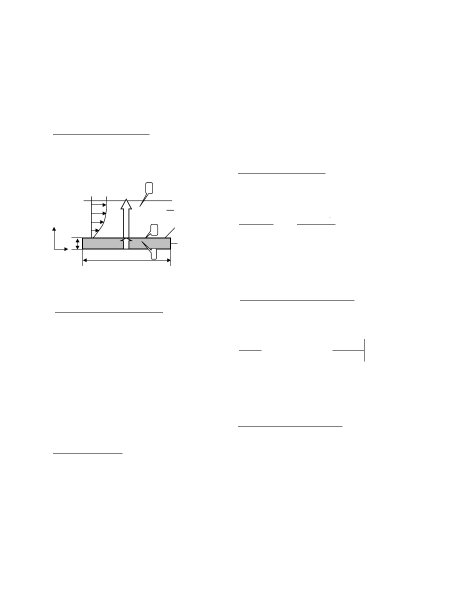
THE EMISSION MODEL

The physical system considered here is a dry building
material (carpet, vinyl flooring, particleboard, etc.) and
has its one surface exposed to the air. The VOC
emission from this material is composed of three main
processes as shown in Figure 1.

Figure 1: Physical configuration of VOC emission from
the dry building material. 1: Internal diffusion; 2:
Material /air interface; 3. External advection.

Mass transfer in the boundary layer
When air passes over the material surface, a mass
boundary layer exists between the surface material and
the main flow. The VOC mass transfer in this mass
boundary layer is determined by diffusion and
convection. The rate of VOC mass transfer in the
boundary layer can be expressed as:

(

)

a

as

C

C

h

R

−

=

(1)

Where h is the mean mass transfer coefficient (m/s), C

as

is the VOC concentration in the air near material
surface (ug/m

3

) and C

a

is the VOC concentration

outside the mass boundary layer (ug/m

3

).

Material /air interface
At the material/air interface, the material is the
adsorbent and the VOC gas is the adsorbate. The
material exerts an attractive force normal to the surface
plane. Consequently, the concentration of VOC at the
material phase exceeds that in the gas phase. Langmuir
and BET are the most common isotherm models which
may be used to describe this process

[11]

. At

atmospheric pressure, for low VOC concentration and
isothermal conditions, equilibrium relation between the

VOC concentration in the air phase and the VOC
concentration in the material phase can be described by
Henry’s law

[12]

:

( )

as

m

kC

t

b

C

=

,

(2)

Where C

m

(b,t) is VOC concentration at the material

surface (ug/m

3

) and C

as

is the VOC concentration in the

air near material surface (ug/m

3

), k is the material/air

partition coefficient, b is the thickness of the material
(m), and t is the time (s).

Mass transfer in the material
For a dry material with homogeneous diffusivity, the
transient VOC diffusion in the material can be
described by the one-dimensional diffusion equation:

( )

( )

2

2

,

,

y

t

y

C

D

t

t

y

C

m

m

m

∂

∂

=

∂

∂

(3)

Where C

m

is the VOC concentration in the material

(ug/m

3

), D

m

is the VOC diffusion coefficient of the

material (m

2

/s) and y is the coordinate in which the

VOC diffusion in the material takes place (m).

Mass balance in the room or chamber
Assuming that the VOC is totally mixed in the room
air. The transient mass balance in the room or chamber
can be expressed by:

( )

( )

b

y

m

m

a

in

a

y

t

y

C

LD

NC

NC

t

t

C

=

∂

∂

−

−

=

∂

∂

,

(4)

Where C

a

is the VOC concentration in the room air

(ug/m

3

), C

in

is the VOC concentration in the supply air

(ug/m

3

), N is the air exchange rate (h

-1

) and L is the

material loading factor (m

2

/m

3

).

Boundary conditions and solutions
Some initial conditions and boundary conditions are
needed to close the above equations.

a) Initial conditions:
A homogeneous new material with initial VOC
concentration of

( )

0

0

,

C

y

C

m

=

(5)

The initial VOC concentration in the room air (C

a0

) is:

b

2

3

a

Air

Boundary
Layer
Interface

Material

y

x

1

( )

0

0

a

a

C

C

=

(6)

b) Boundary conditions:
At the material bottom, there is no VOC passing
through this surface.

( )

0

,

0

=

∂

∂

−

=

y

m

m

y

t

y

C

D

(7)

At the material surface and room air interface, the mass
balance can be written as:

( )

(

)

( )

÷

ø

ö

ç

è

æ

−

=

−

=

∂

∂

−

=

a

m

a

as

b

y

m

m

C

k

t

b

C

h

C

C

h

y

t

y

C

D

,

,

(8)

There are four key parameters which need to be
determined: the mass transfer coefficient in the air, h,
the partition coefficient, k, the mass diffusion
coefficient in the material, D

m

, and the VOC initial

concentration, C

0

.

Mass transfer coefficient in the air, h
In the mass boundary layer, the following relationships
exist

[

13

]

:

a) For laminar flow, (Re

l

<500,000):

2

/

1

3

/

1

Re

664

.

0

l

Sc

Sh

=

(9)

b) For turbulent flow, (Re

l

>500,000):

5

/

4

3

/

1

Re

037

.

0

l

Sc

Sh

=

(10)

c) Combined laminar /turbulent flow, (Re

l

<10

7

,

Re

tr

=500,000):

3

/

1

5

/

4

)

8700

Re

037

.

0

(

Sc

Sh

l

−

=

(11)

Where,

ν

ν

ul

D

Sc

D

hl

Sh

l

a

a

=

=

=

Re

,

,

,

ν

is the

kinematic viscosity of the air (m

2

/s), u is the mean air

velocity over the material (m/s),

l

is the characteristic

length of material (m) and D

a

is the VOC diffusion

coefficient in the air (m

2

/s).

The VOC diffusion coefficient (D

a

) can be directly

obtained from literature

[

14

]

or can be estimated through

other methods. Two main methods have been used to

estimate the VOC diffusion coefficient in the air

[

15

]

:

Fuller, Schettler and Giddings (FSG) method and
Wilke and Lee (WL) method. FSG method is the most
accurate for non-polar gasses at low to moderate
temperatures. In this study, the FGS method was used
to estimate VOC diffusion coefficient in the air. This
method is based on the following correlation:

(

)

2

3

/

1

3

/

1

75

.

1

7

10

VOC

a

r

a

V

V

P

M

T

D

+

=

−

(12)

Where

(

)

VOC

a

VOC

a

r

M

M

M

M

M

+

=

, T is the absolute

temperature (K), P is the pressure (atm), V

a

is the air

molar volume (cm

3

/mol), V

VOC

is the VOC molar

volume (cm

3

/mol), M

a

is the air molecular weight

(g/mol) and M

VOC

is the VOC molecular weight

(g/mol).

Therefore, the mass transfer coefficient can be
estimated using Equations 9-12. Those correlations are
only valid when the concentration at the bottom of
mass boundary layer is constant. Since the VOC
concentration at the material surface is very low and
the VOC diffusion through the material is very slow:
the VOC concentration near the material surface will be
relatively stable. Thus, we may assume that the
concentration near the material surface is constant in a
given time step.

Material/air partition coefficient, k
The material/air partition coefficient describes the
relationship between the concentration in the gas phase
and the concentration in the material phase. It is a
material property and is obtained experimentally

[

5,16

]

.

Mass diffusion coefficient in the material, D

m

The diffusion coefficient in the material is usually a
function of many factors, such as the pore structure, the
material type, compound properties and temperature, as
well as VOC concentration. The dependence of the
diffusion coefficient on the VOC concentration can be
ignored considering that the VOC concentration in the
material is usually very low. The diffusion coefficient
is usually determined experimentally

[

5,16

]

.

Initial concentration, C

0

Initial concentration in the material can be obtained
through solvent extraction, high temperature thermal
desorption or direct analysis

[

17

]

. Recently a cryogenic

grinding/ fluidized bed desorption method was

developed to measure the initial concentration

[

6

]

. The

VOC concentration in the material, VOC emission rate
and the VOC concentration in the room are a function
of the initial concentration, thus a small error in initial
concentration estimation may cause a significant error
in prediction results.

SOLUTION TECHNIQUES

A numerical finite difference method was used to
simultaneously solve equations 1-4 using the initial
conditions, Equations 5 and 6, and boundary
conditions, Equations 7 and 8. The outcomes are:

a) The VOC concentration at the material surface

C

m

(b,t):

(

)

( )

(

)

(

)

(

) (

)

)

13

(

1

,

,

,

1

2

t

t

C

t

Lh

t

N

h

t

t

b

C

t

y

t

y

b

C

y

D

t

b

C

t

Lh

t

N

k

t

Lh

k

h

t

y

y

D

a

m

m

m

m

m

∆

−

+

∆

+

∆

+

∆

−

∆

∆

+

∆

−

∆

=

÷÷ø

ö

ççè

æ

+

∆

+

∆

∆

−

+

∆

∆

+

∆

b) The VOC concentration in the room air, C

a

(t):

( ) (

) ( )

(

) (

)

t

t

C

t

Lh

t

N

t

b

C

t

Lh

t

N

k

t

Lh

t

C

a

m

a

∆

−

+

∆

+

∆

+

+

∆

+

∆

∆

=

1

1

,

1

(14)

c) The VOC emission rate, R(t):

( )

( )

( )

÷

ø

ö

ç

è

æ

−

=

t

C

k

t

b

C

h

t

R

a

m

.

(15)

d) The normalized emitted mass, M/M

0

:

( )

0

1

0

bC

t

t

R

M

M

m

j

å

=

∆

=

(16)

Where

y

∆

is the space grid distance (m),

t

∆

is the

calculation time step (s).

THE MODEL VALIDATION

The model's prediction was compared with the
experimental results of two particleboard tests as well
as the predictions made by a CFD model

[

9

]

.

The model predictions were compared with
experimental data obtained at Massachusetts Institute
of Technology

[9]

. The experiments were carried out in

a small-scale chamber of 0.5

×

0.4

×

0.25 m

3

at a

temperature of 23

±

0.5

0

C, relative humidity 50

±

0.5%,

and air exchange rate 1.0

±

0.05h

-1

. Two different

specimens of particleboard were tested. Major
compounds identified for the tested particleboards were
the same: hexanal,

α

-pinene, camphene, and limonene.

The particleboard properties (D

m

, k, and C

0

) were

estimated by using the chamber emission data
(concentration vs. time) to fit the CFD model

[

9

]

. The

physical properties of the particleboard were supplied
by the experimenter and they are given in Table 1. The
airflow inside the chamber is treated as laminar flow
over a flat plate.

Table 1 Physical properties of particleboard emissions

Compound

TVOC

Hexanal

α

-Pinene

Particleboard 1

D

m

(m

2

/s)

7.65

×

10

-11

7.65

×

10

-11

1.2

×

10

-10

C

0

(ug/m

3

)

5.28

×

10

7

1.15

×

10

7

3.45

×

10

6

k

3289

3289

5602

Particleboard 2

D

m

(m

3

/s)

7.65

×

10

-11

7.65

×

10

-11

1.2

×

10

-10

C

0

(ug/m

3

)

9.86

×

10

7

2.96

×

10

7

7.89

×

10

6

k

3289

3289

5602

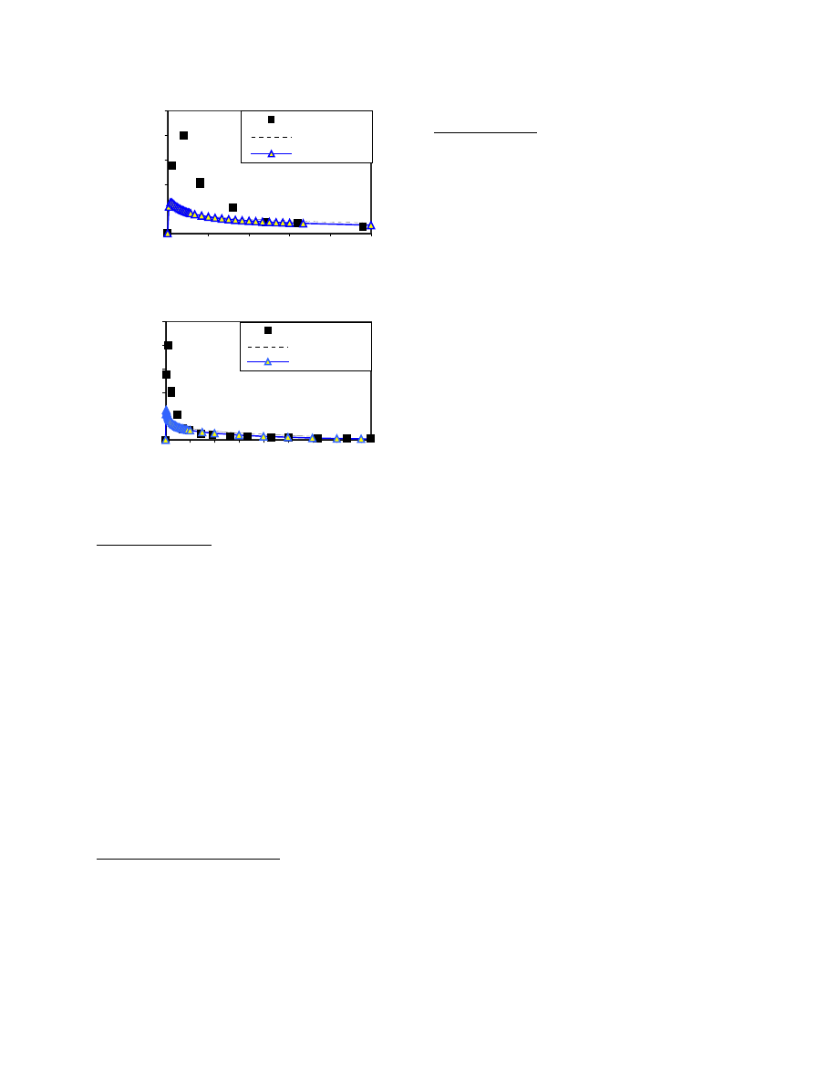
Figures 2 to 7 show the comparison of the predicted
TVOC, hexanal and

α

-pinene concentrations with the

experimental results for particleboard 1. The
experiment was carried out for 96 hours. There is good
agreement between predicted concentrations and
experimental measurements. There are some
discrepancies between predicted results (both with the
proposed numerical model and the CFD model) and
experimental results during the initial hours. This might
be due to instability and partial mixing in the chamber
at the beginning of the tests.

Figures 5 to 7 compare the model predicted TVOC,
hexanal and

α

-pinene concentrations with the

experimental ones for particleboard 2. The experiment
was carried out for 840h in the chamber. As shown in
the figures the predictions of the TVOC, hexanal and

α

-pinene made by the proposed model fit the

experimental data very well. The predicted results and

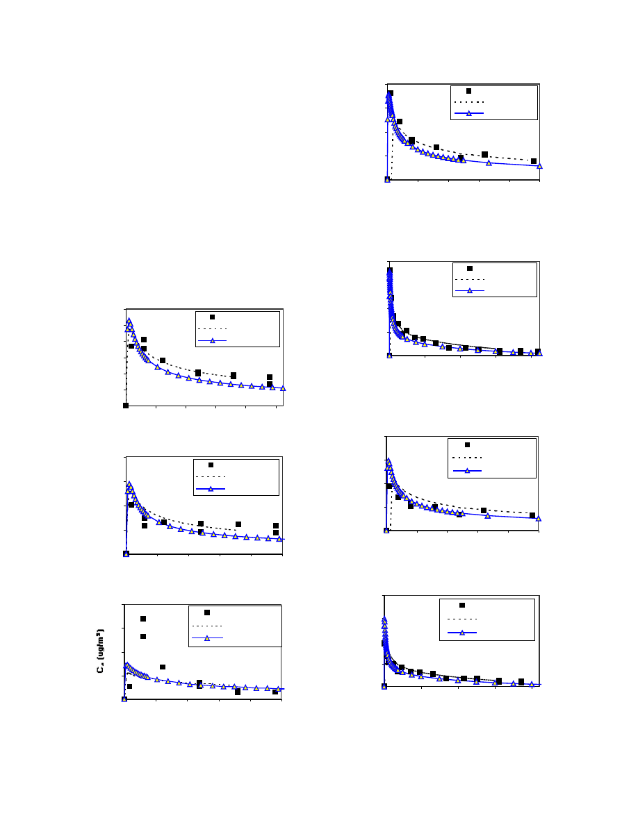
experimental results closely follow the same trend,
especially for the long term; see Figures 5b, 6b and 7b.

The model predictions were also compared with the
prediction of a CFD model

[9]

. Figures 2 to 7 also

compare the model predicted TVOC, hexanal and

α

-

pinene concentrations with the results predicted by a
CFD model. In general, there is excellent agreement
between predicted numerical results, measurement data
and CFD predictions. As shown in Figures 2 and 3, for
short term, the predictions made by CFD for sample 1
(PB1) fit the experimental data better than the proposed
numerical model. While, for long term, Figures 5, 6
and 7 show that the prediction made by the proposed
model fit the experimental data better than the
prediction made by CFD. However, over all, the
predicted curves of the two models follow the
experimental results closely.

0

1000

2000

3000

4000

5000

6000

0

20

40

60

80

100

Time (h)

C

a

(ug/

m

3

)

Measured Data

CFD Model

Numerical model

Figure 2 Comparison of TVOC concentrations (PB1)

0

400

800

1200

1600

0

20

40

60

80

100

Time (h)

C

a

(ug/

m

3)

Measured data

CFD Model

Numerical Model

Figure 3 Comparison of hexanal concentrations (PB1)

0

200

400

600

800

0

20

40

60

80

100

T ime (h)

M easured Data

CFD M odel

Numerical M o del

Figure 4 Comparison of

α

-pinene concentrations (PB1)

0

3,000

6,000

9,000

12,000

0

30

60

90

120

150

Time (h)

C

a

(

ug/m

3

)

Measured Data

CFD Model
numerical Model

Figure 5 (a) Comparison of TVOC concentrations

(PB2)

0

3,000

6,000

9,000

12,000

0

200

400

600

800

Time (h)

C

a

(

ug/

m

3

)

Measured Data

CFD Model
numerical Model

Figure 5 (b) Comparison of TVOC concentrations

(PB2)

0

1,000

2,000

3,000

4,000

0

30

60

90

120

150

Time (h)

C

a

(ug/m

3

)

Measured Data

CFD Model

numerical Model

Figure 6 (a) Comparison of hexanal concentrations

(PB2)

0

1,000

2,000

3,000

4,000

0

200

400

600

800

Time (h)

C

a

(

ug/

m

3

)

Measured Data

CFD Model

numerical Model

Figure 6 (b) Comparison of hexanal concentrations

(PB2)

0

500

1,000

1,500

2,000

2,500

0

30

60

90

120

150

Time (h)

C

a

(ug/m

3

)

Measured Data

CFD Model

numerical Model

Figure 7(a) Comparison of

α

-pinene concentrations

(PB2)

0

500

1,000

1,500

2,000

2,500

0

100 200 300 400 500 600 700 800

Time (h)

C

a

(ug/

m

3

)

Measured Data
CDF Model
nuumerical Model

Figure 7(b) Comparison of

α

-pinene concentrations

(PB2)

CONCLUSIONS

A numerical model was developed to predict the VOC
concentration within the material, the VOC emission
rate and the VOC concentration in the room air. This
model uses four parameters, the diffusion coefficient in
the material (D

m

), material / air partition coefficient (k),

the initial concentration in the material (C

0

) and the

mass transfer coefficient in the air (h). The first three
parameters are properties of the material and can be
determined by experiment, and the last one, h, can be
estimated using fundamentals of fluid dynamics.

The predictions of the model were validated at two
levels: with experimental results from the specially
designed test and with the predictions made by a CFD
model. The results indicate that there is generally good
agreement between the model predictions, the
experimental results and the CFD results.

ACKNOWLEDGEMENTS

This study was supported by a grant from the National
Science and Engineering Research Council Canada and
the EJLB Foundation. We thank Dr. Q. Chen of the
Department of Architecture, Massachusetts Institute of
Technology and Dr. Xudong Yang of the University of
Miami for providing the experimental data.

REFERENCES

1. Haghighat, F., and Bellis, L.D., (1998) ‘Material

emission rates: literature review, and the impact of
indoor air temperature and relative humidity’,
Building and Environment, Vol 33, No 5, pp 261-
277.

2. Tichenor, B.A., Guo, Z. and Sparks, L.E., (1993) ‘

Fundamental mass transfer model for indoor air
emissions from surface coatings’, Indoor Air, 3,
263-268.

3. Spark, L.E., Tichenor, B.A., John C.S. Chang and

Zhishi Guo, (1996) ‘ Gas-phase mass transfer
model for predicting volatile organic compound
emission rates from indoor pollutant sources’,
Indoor Air, 6, 31-40.

4. Haghighat, F. and Zhang, Y. (1999) ‘Modeling of

emission of volatile organic compounds from
building materials-estimation of gas-phase mass
transfer coefficient’, Building and Environment,
Vol. 34, pp. 377-389.

5. Little, J.C. and Hodgson, A.T., (1996) ‘ A Strategy

for Characterizing Homogeneous, Diffusion-
Controlled, Indoor Source and Sinks’, ASTM STP
1287, P294-304.

6. Cox, S.S. Little, J.C., and Hodgson, A.T., (2000), ‘

A new method to predict emission rates of volatile
compounds from vinyl flooring’, Proceeding of
Healthy Building 2000, Vol 4, pp169-174.

7. Lee, C. S., Ghaly, W. and Haghighat, F., (2000), ‘

VOC emission from diffusion controlled building
material: analogy with conjugate heat transfer’,
Proceeding of Healthy Building 2000, Vol 4,
pp163-168.

8. Dunn, J.E. (1987), ‘ Models and statistical methods

for gaseous emission testing of finite sources in
well-mixed chambers’ Atmospheric Environment
21(2), p425-430.

9. Yang, X., Chen, Q., Zhang, J. S., Magee, R., Zeng,

J. and Shaw, C.Y. (2000) ‘Numerical simulation of
VOC emission form dry materials’, Building and
environment. In press.

10. Murakami, S., Kato, S., Kondo, Y., Ito, K., and

Yamamoto, A. (2000), ‘VOC distribution in a
room based on CFD simulation coupled with
emission/ sorption analysis’, Proceeding of the 7

th

international conference on air distribution in
rooms, v. 1, pp 473-478.

11. Masel, R. I., (1996) Principles of adsorption and

reaction on solid surfaces, John Wiley & Sons,
Inc.

12. Axley, J. W., (1991) ‘Adsorption modeling for

building contaminant dispersal analysis’, Indoor
Air, 2, p147-171.

13. White, F. M. (1988), Heat and Mass transfer,

Addison Wesley Series Publishing Company, Inc.

14. Rafson, H., J. (1998) Odor and VOC control

handbook, McGraw-Hill.

15. Layman, W.J. (1982), Handbook of chemical

property estimation methods, New York.

16. Bodalal, A. Zhang, J. S. and Plett, E.G. (2000) ‘ A

method for measuring internal diffusion and
equilibrium partition coefficients of volatile
organic compounds for building materials’,
Building and Environment, p.01-110.

17. Tichenor, B.A. (1996) ‘ Overview of source/sink

characterization methods’, ASTM STP, 1287, p9-
19.