EOS 725 Advanced Hydrosphere

1

Physical Oceanography Notes

Barry A. Klinger

George Mason University

Fall, 2003; Spring, 2006

1

Ekman Layers

1.1

Friction

We wrote that horizontal components of the velocity u = (u, v, w) as a function of (x, y, z, t)
are governed by the momentum equations,

Du

Dt

− f v = −

1
ρ

∂p

∂x

+ F

x

(1a)

Dv

Dt

+ f u = −

1
ρ

∂p
∂y

+ F

y

.

(1b)

Note that boldface symbols (such as u) represent vectors. Now we will consider the effects

of friction, which we ignored up to this point.

Just as temperature and salinity diffuse through a fluid, so does momentum. Therefore

we can think of friction as the diffusion of momentum. If we have an isolated current,
some of the momentum represented by the flow will spread out into neighboring, unmoving
fluid. In laminar flow—relatively simple flow which does not have turbulent motion—this
momentum diffusion is due to the random movement of molecules inside the fluid. The rate
at which momentum spreads is set by a property of the fluid, the kinematic viscosity ν.
For water in oceanographically relevant temperature ranges, ν is approximately constant.
Mathematically, the diffusion law can be written

F

x

= ν∇

2

u

(2a)

F

y

= ν∇

2

v

(2b)

The molecular viscosity is actually so small that it is irrelevant in the real ocean.

Random molecular motion is simply not an efficient way to transmit momentum hundreds of
meters in the vertical or hundreds of kilometers in horizontal directions. Instead, turbulent
motion on length scales ranging from mm to hundreds (even thousands) of meters spreads out
momentum. We can characterize this diffusion with an “eddy viscosity” which is generally
very different in the vertical (ν

V

) and horizontal (ν

H

) directions and which varies drastically

EOS 725 Advanced Hydrosphere

2

throughout the ocean depending on conditions such as forcing, topography, and velocity.
There is much we don’t know about this kind of momentum mixing, but it is still convenient
to approximate the mixing as a diffusion law

F

x

= ν

V

∂

2

u

∂x

2

+ ν

H

∇

2

H

u

(3a)

F

y

= ν

V

∂

2

v

∂y

2

+ ν

H

∇

2

H

v,

(3b)

where ∇

2

H

includes only the horizontal components of ∇

2

.

1.2

Wind Stress Without, and With, Rotation

We often think of friction as a force which causes a system to lose momentum, and friction
in the ocean plays an important role in “braking” ocean currents. In addition, friction can
also impart momentum to a system, as when one pushes down on a piece of paper and slides
it across a table. In the ocean, a major source of energy for ocean currents is frictional stress
from wind blowing over the ocean’s surface. Earlier we discussed pressure, which is the
force/area normal to a given surface. The stress, τ , is the force/area tangent to a surface.
The stress can be thought of as the flux of momentum across a surface. The horizontal
components of stress—that is, the vertical flux of horizontal momentum—can be written

τ = ρν

∂u

∂z

.

(4)

The wind stress is related to the speed of the wind. Typically the stress is proportional

to the speed squared. While it is not trivial to measure wind stress, windstress over the
ocean is routinely estimated to an accuracy of about 20%, and so it is useful to think of
wind stress as given and try to understand how the ocean would respond to this wind stress.
Mathematically, the wind stress is part of the boundary conditions governing equation (1).
We also need a boundary condition for the bottom boundary (the ocean floor). Here the
stress is not generally known, but we do know from general fluid dynamics principles that
u = 0 at the bottom. This is also the same boundary condition for the bottom of atmosphere.
The boundary conditions for top and bottom of the ocean thus look somewhat different from
each other. However, we will see below that both boundaries have some similar features.

To understand the influence of wind stress, we look at a simplified situation in which

we take τ , u, and p to be uniform in x and y (but can vary in z) and constant in time.
This assumes that if we start the wind and then wait for it to blow long enough, the system
will eventually reach some steady state. In equation (1), this eliminates inertia and pressure

EOS 725 Advanced Hydrosphere

3

forces. Using equation (3) for the pressure forces, (1) becomes simply

−f v = ν

V

∂

2

u

∂z

2

(5a)

f u = ν

V

∂

2

v

∂z

2

(5b)

In the nonrotating case, we would expect that the frictional effect of wind would

extend all the way down the water column to the bottom of the ocean. This can be shown
by solving (5) in the relatively simple case of f = 0, subject to boundary conditions of a
given stress τ at the surface and u = 0 at the bottom. For the nonrotating case, something
peculiar happens: if one solves the f 6= 0 case mathematically (somewhat tedious but still
not too hard to do), one finds that the region of frictional influence is confined to a region
above a depth D, where D depends on ν

V

and f . A similar region of frictional influence

exists on the bottom, if we assume there is some “background” u which is slowed by friction
close to the bottom. In either case, the region of frictional influence is called the Ekman
layer.

1.3

Properties of the Ekman Layer

For a laminar surface Ekman layer (constant ν

V

), the velocity not only decreases with depth,

but also changes direction. The velocity at the surface is 45

◦

to the right (in the Northern

Hemisphere) of the τ vector, but far enough down the velocity is actually in the opposite
direction. This velocity profile is known as an Ekman spiral.

In the real ocean, with complicated (and poorly-known) ν

V

, the behavior is not exactly

the same as the theoretical Ekman spiral. *[ Usually the Ekman layer thickness D is about
the same as the mixed layer thickness. D is often assumed to be no more than about 50 m,
even when the mixed layer is much deeper. ]*In any case, there is a robust feature of the
wind-driven flow that is independent of the details of ν

V

. First, it is useful to define a kind

of transport vector,

U

E

= (U

E

, V

E

) =

Z

0

−D

udz

(6)

where here we define u = (u, v) rather than (u, v, w). In class we defined a volume trans-
port, which was velocity times an area and had units of volume/time. U is similar but
is a velocity times a length, with units of area/time. It would be logical to call it an area
transport, but no one ever does. Because in this case it is a measure of the total wind-driven
horizontal flow at a particular (x, y) position, it is called the Ekman transport.

EOS 725 Advanced Hydrosphere

4

τ

F

p

U

E

x

y

(1a) Wind−Driven Ekman Layer

u

F

p

τ

U

E

x

y

(1b) Bottom Ekman Layer

Now we can simplify (5) by taking

R

0

−D

dz of it, where z = 0 is the upper surface of

the ocean. This gives us

−f V = ν

V

∂u

∂z

|

0

−D

(7a)

f U = ν

V

∂v
∂z

|

0

−D

.

(7b)

The equations are simpler in this form because we know that ∂u/∂z is related to the wind

stress (eq 4) at the surface and goes to zero at the bottom of the Ekman layer. Therefore,
if we define the wind stress components τ = (τ, σ), (7) can be rewritten

V = −

τ

ρf

(8a)

U =

σ

ρf

(8b)

As promised, this allows us to calculate the total horizontal flow in the Ekman layer if we

know the windstress, density (which is approximately the same everywhere in the ocean),
and the Coriolis parameter f (which is a known function of latitude).

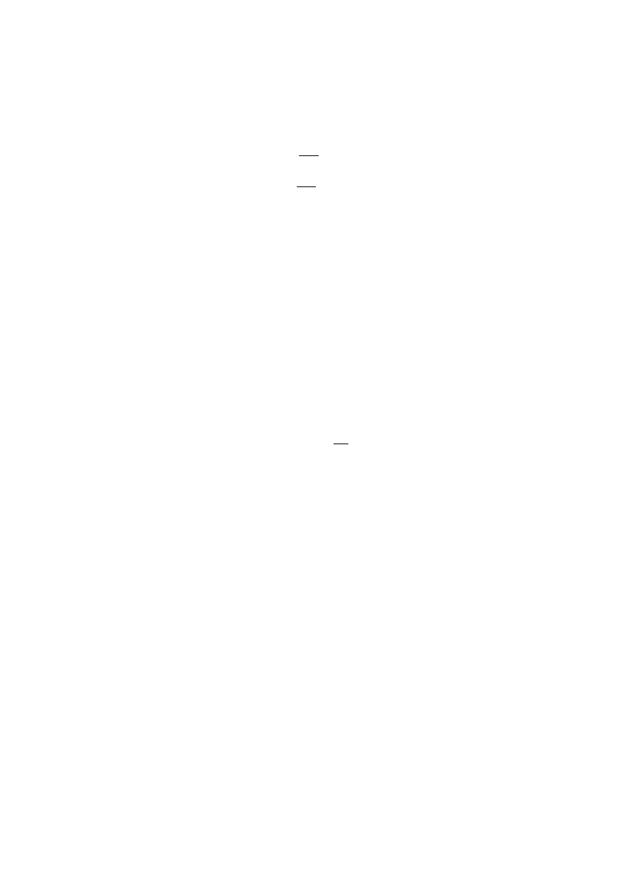
The wind-driven Ekman transport is always perpendicular to the wind stress direc-

tion (to the right in the northern hemisphere, to the left in the southern). The relationship
between the forces and the Ekman transport can be summarized by a simple diagram (Fig-
ure 1a). In the Ekman layer, the force due to wind stress is balanced by the Coriolis force, so
given τ , we know that the Coriolis force F

p

is equal and opposite. Since the Coriolis force is

always 90

◦

to the right (northern hemisphere) of the velocity, this immediately tells us which

EOS 725 Advanced Hydrosphere

5

way the Ekman transport is going. Note that this only applies to the Ekman transport; the
actual velocity at different depths within the Ekman layer points in different directions as
discussed above.

A similar force diagram can be written for the bottom Ekman layer. Here we assume

that there is some uniform velocity above the Ekman layer (Figure 1b). Friction in the Ekman
layer makes a bottom stress τ in the opposite direction to the velocity. As in Figure 1a, we
deduce an equal and opposite F

p

and an associated U

E

at right angles to it.

1.4

Ekman Pumping

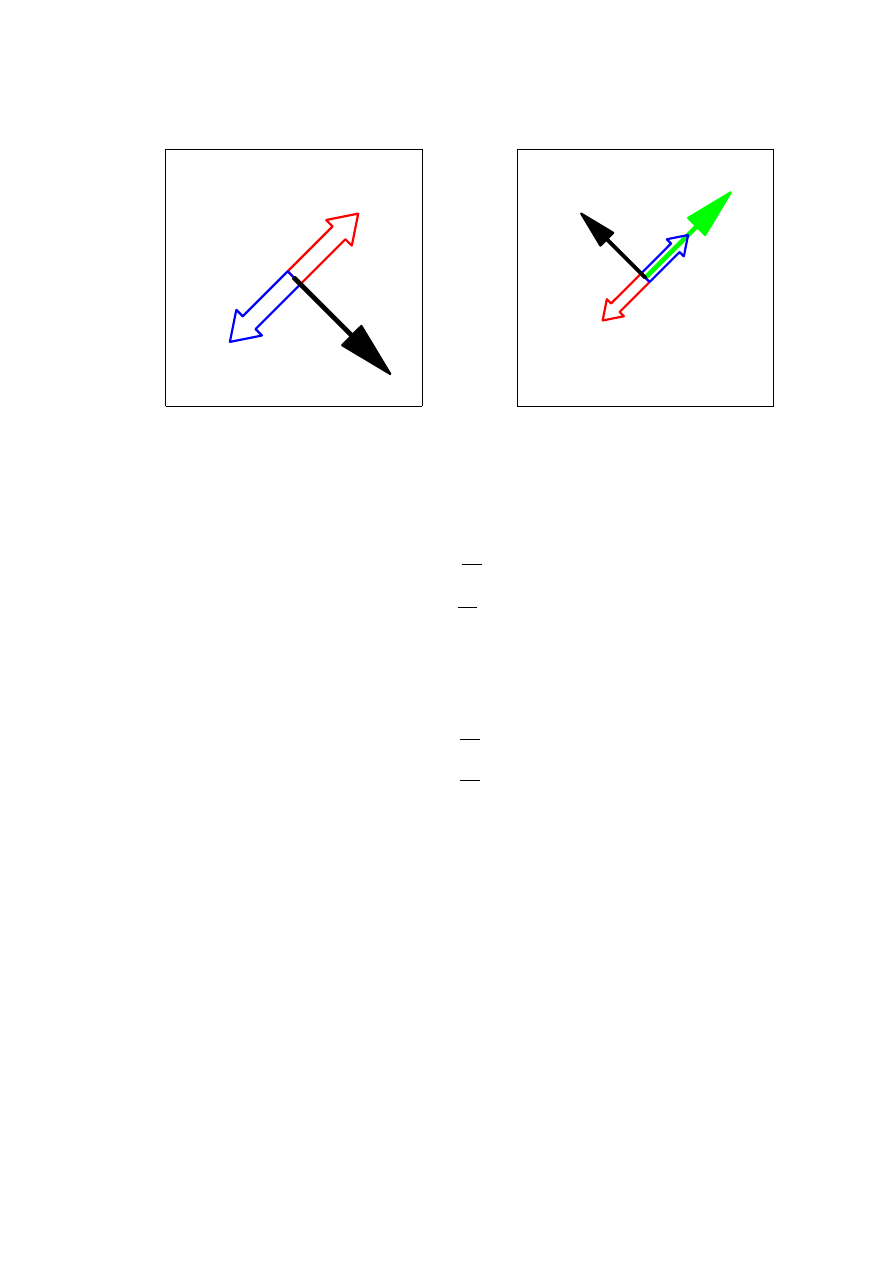
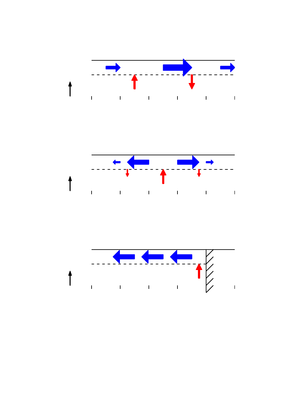
Surface stress not only induces horizontal velocity in the ocean, it can also cause vertical
flow as well. This occurs whenever there is a divergence of Ekman transport: that is, more
flow enters a region than leaves it. This is illustrated by several examples in Figure 2.
Mathematically, the upwelling or downwelling induced by the horizontal divergence can be
calculated from the incompressibility condition:

∇

H

· u + ∂w/∂z = 0.

(9)

Taking

R

0

−D

of (9), using the definition of the Ekman transport, and assuming that w(z =

0) = 0 (no flow through the top of the ocean), we obtain

w(z = −D) = ∇

H

· U

E

.

(10)

Ekman pumping is important to the ocean biota. Often the amount of phytoplanck-

ton, which form the base of the food chain, is determined by the availability of nutrients near
the sea surface (where light penetrates). Nutrients tend to rain out of the surface layer as
fecal pellets or other detritus. Ocean upwelling can bring these nutrients back up, increasing
biological productivity, while downwelling decreases productivity. Coastal and equatorial
upwelling can be particularly strong, and these regions have especially high productivity.

EOS 725 Advanced Hydrosphere

6

sea surface

Ekman layer

latitude

30

35

40

45

50

55

z

upwelling

downwelling

Ekman
Transport

(2a)

τ

and f Both Vary

sea surface

Ekman layer

latitude

−10

−6

−2

2

6

10

z

upwelling

downwelling

downwelling

(2b)

τ

uniform, f varies

sea surface

Ekman layer

land

relative longitude

−8

−6

−4

−2

0

2

z

upwelling

(2c)

τ

Uniform, Coastal Upwelling