
© 2001 by CRC Press LLC
1
Three-Dimensional
Dynamic Anatomical
Modeling of the
Human Knee Joint
Biomechanical Systems • Physical Knee Models •
Phenomenological Mathematical Knee Models • Anatomically
Based Mathematical Knee Models
Three-Dimensional Dynamic Modeling of the
Tibio-Femoral Joint: Model Formulation
Kinematic Analysis • Contact and Geometric Compatibility
Conditions • Ligamentous Forces • Contact Forces • Equations
of Motion
DAE Solvers • Load Vector and Stiffness Matrix
Varus-Valgus Rotation • Tibial Rotation • Femoral and Tibial
Contact Pathways • Velocity of the Tibia • Magnitude of the
Tibio-Femoral Contact Forces • Ligamentous Forces
Three-dimensional dynamic anatomical modeling of the human musculo-skeletal joints is a versatile tool
for the study of the internal forces in these joints and their behavior under different loading conditions
following ligamentous injuries and different reconstruction procedures. This chapter describes the three-
dimensional dynamic response of the tibio-femoral joint when subjected to sudden external pulsing loads
utilizing an anatomical dynamic knee model. The model consists of two body segments in contact (the
femur and the tibia) executing a general three-dimensional dynamic motion within the constraints of
the ligamentous structures. Each of the articular surfaces at the tibio-femoral joint is represented by a
separate mathematical function. The joint ligaments are modeled as nonlinear elastic springs. The six-
degrees-of-freedom joint motions are characterized using six kinematic parameters and ligamentous
forces are expressed in terms of these six parameters. In this formulation, all the coordinates of the
ligamentous attachment points are dependent variables which allow one to easily introduce more liga-
ments and/or split each ligament into several fiber bundles. Model equations consist of nonlinear second
order ordinary differential equations coupled with nonlinear algebraic constraints. An algorithm was
developed to solve this differential-algebraic equation (DAE) system by employing a DAE solver, namely,
the Differential Algebraic System Solver (DASSL) developed at Lawrence Livermore National Laboratory.
Mohamed Samir Hefzy
University of Toledo
Eihab Muhammed Abdel-
Rahman
Virginia Polytechnic Institute

© 2001 by CRC Press LLC
Model calculations show that as the knee was flexed from 15 to 90°, it underwent internal tibial
rotation. However, in the first 15° of knee flexion, this trend was reversed: the tibia rotated internally
as the knee was extended from 15° to full extension. This indicates that the screw-home mechanism
that calls for external rotation in the final stages of knee extension was not predicted by this model.
This finding is important since it is in agreement with the emerging thinking about the need to re-
evaluate this mechanism.
It was also found that increasing the pulse amplitude and duration of the applied load caused a decrease
in the magnitude of the tibio-femoral contact force at a given flexion angle. These results suggest that
increasing load level caused a decrease in joint stiffness. On the other hand, increasing pulse amplitude
did not change the load sharing relations between the different ligamentous structures. This was expected
since the forces in a ligament depend on its length which is a function of the relative position of the tibia
with respect to the femur.
Reciprocal load patterns were found in the anterior and posterior fibers of both anterior and posterior
cruciate ligaments, (ACL) and (PCL), respectively. The anterior fibers of the ACL were slack at full
extension and tightened progressively as the knee was flexed, reaching a maximum at 90° of knee flexion.
The posterior fibers of the ACL were most taut at full extension; this tension decreased until it vanished
around 75° of knee flexion. The forces in the anterior fibers of the PCL increased from zero at full
extension to a maximum around 60° of knee flexion, and then decreased to 90° of knee flexion. On the
other hand, the posterior fibers of the PCL were found to carry lower loads over a small range of motion;
these forces were maximum at full extension and reached zero around 10° of knee flexion. These results
suggest that regaining stability of an ACL deficient knee would require the reconstruction of both the
anterior and posterior fibers of the ACL. On the other hand, these data suggest that it might be sufficient
to reconstruct the anterior fibers of the PCL to regain stability of a PCL deficient knee.
1.1 Background
Biomechanical Systems
Biomechanics is the study of the structure and function of biological systems by the means of the methods
of mechanics.
63
Biomechanics thus provides the means to study and analyze the behaviors of the different
biological systems as well as their components. Models have emerged as necessary and effective tools to
be employed in the analysis of these biomechanical systems.
In general, employing models in system analysis requires two prerequisites: a clear objective identifying
the aims of the study, and an explicit specification of the assumptions to be made. A system mainly
depends upon what it is being used to determine, e.g., joint stiffness or individual ligament lengths and
forces. The system is thus identified according to the aim of the study. Assumptions are then introduced
in order to simplify the system and construct the model. These assumptions also depend on the aim of
the study. For example, if the intent is to determine the failure modes of a tendon, it is not reasonable
to model the action of a muscle as a single force applied to the muscle’s attachement point. On the other
hand, this assumption is appropriate if it is desired to determine the effect of a tendon transfer on gait.
After the system has been defined and simplified, the modeling process continues by identifying system
variables and parameters. The parameters of a system characterize its components while the variables
describe its response. The variables of a system are also referred to as the quantities being determined.
Modeling activities include the development of physical models and/or mathematical models. The
mechanical responses of physical models are determined by conducting experimental studies on fabri-
cated structures to simulate some aspect of the real system. Mathematical models satisfy some physical
laws and consist of a set of mathematical relations between the system variables and parameters along
with a solution method. These relations satisfy the boundary and initial conditions, and the geometric
constraints.
Major problems can be encountered when solving the mathematical relations forming a mathematical
model. They include indeterminacy, nonlinearity, stability, and convergence. Several procedures have

© 2001 by CRC Press LLC
been developed to overcome some of these difficulties. For example, eliminating indeterminacy requires
using linear or nonlinear optimization techniques. Different numerical algorithms
16
presented in the
literature effectively allow solution of most nonlinear systems of equations, yet reaching a stable and
convergent solution never may be achieved in some situations. However, with the recent advances in
computers, mathematical models have proved to be effective tools for understanding behaviors of various
components of the human musculo-skeletal system.
Mathematical models are practical and appealing because:
1. For ethical reasons, it is necessary to test hypotheses on the functioning of the different components
of the musculo-skeletal system using mathematical simulation before undertaking experimental
studies.
115
2. It is more economical to use mathematical modeling to simulate and predict joint response under
different loading conditions than costly
in vivo
and/or
in vitro
experimental procedures.
3. The complex anatomy of the joints means it is prohibitively complicated to instrument them or
study the isolated behaviors of their various components.
4. Due to the lack of noninvasive techniques to conduct
in vivo
experiments, most experimental
work is done
in vitro
.
This chapter focuses on the human knee joint which is one of the largest and most complex joints
forming the musculoskeletal system. From a mechanical point of view, the knee can be considered as a
biomechanical system that comprises two joints: the tibio-femoral and the patello-femoral joints. The
behavior of this complicated system largely depends on the characteristics of its different components.
As indicated above, models can be physical or mathematical. Review of the literature reveals that few
physical models have been constructed to study the knee joint. Since this book is concerned with
techniques developed to study different biomechanical systems, the few physical knee models will be
discussed briefly in this background section.
Physical Knee Models
Physical models have been developed to determine the contact behavior at the articular surfaces and/or
to simulate joint kinematics. In order to analyze the stresses in the contact region of the tibio-femoral
joint, photoelasticity techniques have been employed in which epoxy resin was used to construct models
of the femur and tibia.
31,87
Kinematic physical knee models were also proposed to demonstrate the
complex tibio-femoral motions that can be described as a combination of rolling and gliding.
100,101
The most common physical model that has been developed to illustrate the tibio-femoral motions is
the crossed four-bar linkage.
76,88,89
This construct consists of two crossed rods that are hinged at one end
and have a length ratio equal to that of the normal anterior and posterior cruciate ligaments. The free
ends of these two crossed rods are connected by a coupler that represents the tibial plateau. This simple
apparatus was used to demonstrate the shift of the contact points along the tibio-femoral articular surfaces
that occur during knee flexion.
Another model, the Burmester curve, has been used to idealize the collateral ligaments.
90
This curve
is comprised of two third order curves: the vertex cubic and the pivot cubic. The construct combining
the crossed four-bar linkage and the Burmester curve has been used extensively to gain an insight into
knee function since the cruciate and collateral ligaments form the foundation of knee kinematics.
However, this model is limited because it is two-dimensional and does not bring tibial rotations into the
picture. A three-dimensional model proposed by Huson allows for this additional rotational degree-of-
freedom.
76
Phenomenological Mathematical Knee Models
Several mathematical formulations have been proposed to model the response of the knee joint which
constitutes a biomechanical system. Three survey papers appeared in the last decade to review

© 2001 by CRC Press LLC
mathematical knee models which can be classified into two types:
phenomenological
and
anatomically
based
models.
66,69,70
The phenomenological models are gross models, describing the overall response of the knee without
considering its real substructures. In a sense, these models are not real knee models since a model’s
effectiveness in the prediction of
in vivo
response depends on the proper simulation of the knee’s
articulating surfaces and ligamentous structures. Phenomenological models are further classified into
simple hinge
models, which consider the knee a hinge joint connecting the femur and tibia, and
rheological
models, which consider the knee a viscoelastic joint.
Simple Hinge Models
This type of knee model is typically incorporated into global body models. Such whole-body models
represent body segments as rigid links connected at the joints which actively control their positions.
Some of these models are used to calculate the contact forces in the joints and the muscle load sharing
during specific body motions such as walking,
38,73,86,112,114
running,
25
and lifting and lowering tasks.
39,44
These models provide no details about the geometry and material properties of the articular surfaces
and ligaments. Equations of motion are written at the joint and an optimization technique is used to
solve the system of equations for the unknown muscle and contact forces. Other simple hinge models
were developed to predict impulsive reaction forces and moments in the knee joint under the impact of
a kick to the leg in the sagittal plane.
83,121,122
In these models, the thigh and the leg were considered as a
double pendulum and the impulse load was expressed as a function of the initial and final velocities of
the leg.
Rheological Models
These models use linear viscoelasticity theory to model the knee joint using a Maxwell fluid
approximation
97
or a Kelvin body idealization.
37,108
Masses, springs, and dampers are used to represent
the velocity-dependent dissipative properties of the muscles, tendons, and soft tissue at the knee joint.
These models do not represent the behavior of the individual components of the knee; they use exper-
imental data to determine the overall properties of the knee. While phenomenological models are of
limited use, their dynamic nature makes them of interest.
Anatomically Based Mathematical Knee Models
Anatomically based models are developed to study the behaviors of the various structural components
forming the knee joint. These models require accurate description of the geometry and material properties
of knee components. The degree of sophistication and complexity of these models varies as rigid or
deformable bodies are employed. The analysis conducted in most of the knee models employs a system
of rigid bodies that provides a first order approximation of the behaviors of the contacting surfaces.
Deformable bodies have been introduced to allow for a better description of this contact problem.
Employing rigid or deformable bodies to describe the three-dimensional surface motions of the
tibia and/or the patella with respect to the femur using a mathematical model requires the development
of a three-dimensional mathematical representation of the articular surfaces. Methods include describ-
ing the articular surfaces using a combination of geometric primitives such as spheres, cones, and
cylinders,
4-7,116,125,136,137
describing each of the articular surfaces by a separate polynomial function of
the form y = y (x, z),
21,23,75
and describing the articular surfaces utilizing the piecewise continuous
parametric bicubic Coons patches.
12,14,67,68
The B-spline least squares surface fitting method is also used
to create such geometric models.
13
Hefzy and Grood
66
further classified anatomically based models into
kinematic
and
kinetic
models.
Kinematic models describe and establish relations between motion parameters of the knee joint. They
do not, however, relate these motion parameters to the loading conditions. Since the knee is a highly
compliant structure, the relations between motion parameters are heavily dependent on loading condi-
tions making each of these models valid only under a specific loading condition. Kinetic models try to
remedy this problem by relating the knee’s motion parameters to its loading condition.

© 2001 by CRC Press LLC
In turn kinetic models are classified as
quasi-static
and
dynamic
. Quasi-static models determine forces
and motion parameters of the knee joint through solution of the equilibrium equations, subject to
appropriate constraints, at a specific knee position. This procedure is repeated at other positions to cover
a range of knee motion. Quasi-static models are unable to predict the effects of dynamic inertial loads
which occur in many locomotor activities; as a result, dynamic models have been developed. Dynamic
models solve the differential equations of motion, subject to relevant constraints, to obtain the forces
and motion parameters of the knee joint under dynamic loading conditions. In a sense, quasi-static
models march on a space parameter, for example, flexion angle, while dynamic models march on time.
Quasi-Static Anatomically Based Knee Models
Several three-dimensional anatomical quasi-static models are cited in the literature. Some of these models
are for the tibio-femoral joint, some for the patello-femoral joint, some include both tibio-femoral and
patello-femoral joints, and some include the menisci. The most comprehensive quasi-static models for
the tibio-femoral joint include those developed by Wismans et al.,
129,130
Andriacchi et al.,
9
and Blankevoort
et al.
20-23
The most comprehensive quasi-static three-dimensional models for the patello-femoral joint
include those developed by Heegard et al.,
64
Essinger et al.,
50
Hirokawa,
72
and Hefzy and Yang.
68
The
models developed by Tumer and Engin,
118
Gill and O’Connor,
57
and Bendjaballah et al.
17
are the only
models that realistically include both tibio-femoral and patello-femoral joints. The latter model is the
only and most comprehensive quasi-static three-dimensional model of the knee joint available in the
literature.
17
This model includes menisci, tibial, femoral and patellar cartilage layers, and ligamentous
structures. The bony parts were modeled as rigid bodies. The menisci were modeled as a composite of
a matrix reinforced by collagen fibers in both radial and circumferential directions. However, this com-
prehensive model is limited because it is valid only for one position of the knee joint: full extension.
This chapter is devoted to the dynamic modeling of the knee joint. Therefore, the previously cited
quasi-static models will not be further discussed. The reader is referred to the review papers on knee
models by Hefzy et al. for more details on these quasi-static models.
66,70
Dynamic Anatomically Based Knee Models
Most of the dynamic anatomical models of the knee available in the literature are two-dimensional,
considering only motions in the sagittal plane. These models are described by Moeinzadeh et al.,
93-99
Engin and Moeinzadeh,
47
Wongchaisuwat et al.,
131
Tumer et al.,
118-119
Abdel-Rahman and Hefzy,
1-3
and
Ling et al.
84
Moeinzadeh et al.’s two-dimensional model of the tibio-femoral joint represented the femur and the
tibia by two rigid bodies with the femur fixed and the tibia undergoing planar motion in the sagittal
plane.
93,96
Four ligaments, the two cruciates and the two collaterals were modeled by a spring element
each. Ligamentous elements were assumed to carry a force only if their current lengths were longer than
their initial lengths, which were determined when the tibia was positioned at 54.79° of knee flexion. A
quadratic force elongation relationship was used to calculate the forces in the ligamentous elements. A
one contact point analysis was conducted where normals to the surfaces of the femur and the tibia, at
the point of contact, were considered colinear. The profiles of the femoral and tibial articular surfaces
were measured from X-rays using a two-dimensional sonic digitizing technique. A polynomial equation
was generated as an approximate mathematical representation of the profile of each surface. Results were
presented for a range of motion from 54.79° of knee flexion to full extension under rectangular and
exponential sinusoidal decaying forcing pulses passing through the tibial center of mass. No external
moments were considered in the numerical calculation.
Moeinzadeh et al.’s theoretical formulation included three differential equations describing planar
motion of the tibia with respect to the femur, and three algebraic equations describing the contact
condition and the geometric compatibility of the problem.
93-96
Using Newmark’s constant-average-accel-
eration scheme,
15
the three differential equations of motion were transformed to three nonlinear algebraic
equations. Thus, the system was reduced to six nonlinear algebraic equations in six independent
unknowns: the
x
and
y
coordinates of the origin of the tibial coordinate system with respect to the femoral

© 2001 by CRC Press LLC
system, the angle of knee flexion, the magnitude of the contact force, and the
x
coordinates of the contact
point in both the femoral and tibial coordinate systems. However, instead of using the differential form
of the Newton-Raphson iteration technique to solve these six nonlinear algebraic equations in their
numerical analysis, Moeinzadeh et al. used an incremental form of the Newton-Raphson technique. Thus,
they reformulated the system of equations to include 22 equations in 22 unknowns. This system was
solved iteratively. In this formulation they considered the coordinates of the ligamentous tibial insertion
sites (moving points) as eight independent variables and added eight compatibility equations for the
locations of these ligamentous tibial insertion sites. The remaining independent variables included
1. The
x
and
y
components of the unit vectors normal to the femoral and to the tibial profiles at the
point of contact (four variables)
2. The
y
coordinates of the contact point in both the femoral and tibial coordinate systems (two
variables)
3. The slope of the articular profiles at the contact point expressed in both femoral and tibial
coordinate systems (two variables)
Moeinzadeh et al.’s model was limited since it was valid only for a range of 0° to 55° of knee flexion.
This limitation was a result of their mathematical representation of the femoral profile that diverged
significantly from the anatomical one in the posterior part of the femur and their assumption that all
ligaments were only taut at 54.79° of knee flexion.
Moeinzadeh et al. extended their work and presented a formulation for the three-dimensional version
of their model. However, they were not able to obtain a solution because of “... the extreme complexity
of the equations
.
” Their solution technique required them to consider an additional 85 variables as
independent and add 85 compatibility equations to solve a system of 101 equations in 101 unknowns.
Wongchaisuwat et al.
131
presented a dynamic model to analyze the planar motion between the femoral
and tibial contact surfaces in the sagittal plane. In their model, the authors considered the tibia as a
pendulum that swings about the femur. Newton’s and Euler’s equations of motion were then used to
formulate the gliding and rolling motions defined by holonomic and nonholonomic conditions, respec-
tively. Using their model, the authors presented a control strategy to cause the motion and maintain the
contact between the surfaces. Their control system included two classes of input: muscle forces, which
caused and stabilized the motion, and ligament forces, which maintained the constraints.
To investigate the applicability of classical impact theory to an anatomically based model of the tibio-
femoral joint, Engin and Tumer
48,49
developed a modified version of Moeinzadeh et al.’s model. Unstrained
lengths of the ligaments were calculated by assuming strain levels at full extension. The model used a
two-piece force-elongation relationship, including linear and quadratic regions, to evaluate the ligamen-
tous forces. Engin and Tumer proposed two improved methods to obtain the response of the knee joint
using this model. These are the minimal differential equation (MDE) and the excess differential equation
(EDE) methods.
In the MDE method, the algebraic equations (constraints) are eliminated through their use to express
some variables in terms of others in closed form. Furthermore, one of the differential equations of motion
is used to express the contact force in terms of the other variables. It is then used in the other differential
equations to eliminate the contact force from the differential equations system, thus reducing that system
by one equation. The resulting nonlinear ordinary differential equation system is then solved using both
Euler and Runge-Kutta methods of numerical integration.
In the EDE method, the algebraic constraints are converted to differential equations by differentiating
them twice with respect to time, producing a second order ordinary differential equation system in the
position parameters (five variables). One equation of motion is dropped from the system of equations
and used to express the magnitude of the contact force in terms of the other variables. The system is
thus reduced to a system of five differential equations in five unknowns. This system of equations is then
integrated numerically using both Euler and Runge-Kutta methods of numerical integration. Upon
evaluating the position parameters, the last equation of motion is solved for the contact force. The basic

© 2001 by CRC Press LLC
assumption in this method is that if the constraints are satisfied initially, then satisfying the second
derivatives of the constraints in future time steps is expected to satisfy the constraints themselves.
Tumer and Engin
118
extended the Engin and Tumer model
48,49
to include both the tibio-femoral and
the patello-femoral joints and introduced a two-dimensional, three-body segment dynamic model of the
knee joint. The model incorporated the patella as a massless body and the patellar ligament as an
inextensible link. At each time step of the numerical integration, the system of equations governing the
tibio-femoral joint was solved using the MDE method, then the system of equations governing the motion
of the patello-femoral joint, a non-linear algebraic equations system, was solved using the Newton-
Raphson method.
Abdel-Rahman and Hefzy presented a modified version of Moeinzadeh et al.’s model.
1-4
A part of a
circle was used to represent the profile of the femur and a parabolic polynomial was used to represent
the tibia. Ten ligamentous elements were used to model the major knee ligaments and the posterior fibers
of the capsule. The unstrained lengths of the ligamentous elements were calculated by assuming strain
levels at full extension. A quadratic force elongation relationship was used to evaluate the ligamentous
forces. Results were obtained for knee motions under a sudden impact simulated by a posterior forcing
pulse in the form of a rectangular step function applied to the tibial center of gravity when the knee joint
was at full extension; knee motions were tracked until 90° knee flexion was achieved. The results
demonstrated the effects of varying the pulse amplitude and duration on the velocity and acceleration
of the tibia, as well as on the magnitude of the contact force and on the different ligamentous forces.
Furthermore, Abdel-Rahman and Hefzy introduced another approach, the reverse EDE method, to
solve the two-dimensional dynamic model of the tibio-femoral joint.
1-4
In the reverse EDE method, the
Newmark method is used to transform the differential equations of motion into non-linear algebraic
equations. Combining these equations with the non-linear algebraic constraints, the resulting nonlinear
algebraic system of equations is solved using the differential form of the Newton-Raphson method.
In Moeinzadeh et al.’s formulation, the coordinates of the ligaments’ insertion sites were considered
as independent variables. This approach caused the model to become more complicated when more
ligaments were introduced or existing ligaments were subdivided into several elements. This major
problem was solved by the Abdel-Rahman and Hefzy formulation in which all the coordinates of the
ligaments’ insertion sites were considered as dependent variables. As a result, introducing more ligaments
to the model or splitting existing ligaments into several fiber bundles to better represent them did not
affect the system to be solved. Furthermore, Abdel-Rahman and Hefzy used a more anatomical femoral
profile, enabling them to predict tibio-femoral response over a range of motion from 0 to 90° of knee
flexion.
1-3
In summary, since Wongchaisuwat et al.’s model
131
is more a control strategy to cause and maintain
contact between the femur and the tibia, it is not considered a real mathematical model that predicts
knee response under dynamic loading. Most of the remaining dynamic models
1-3,47-49,93-96
can be perceived
as different versions of a single dynamic model. Such a model is comprised of two rigid bodies: a fixed
femur and a moving tibia connected by ligamentous elements and having contact at a single point. The
various versions of this model have severe limitations in that they are two-dimensional in nature. A three-
dimensional dynamic version of the model was presented by Moeinzadeh and Engin.
98
However, obtain-
ing results using their formulation was not possible because of the limitations of the solution technique.
In this chapter, we present the three-dimensional version of this dynamic model. A new approach, the
modified reverse EDE method is presented and used to solve the governing system of equations. In this
solution technique, the second order time derivatives are first transformed to first order time derivatives
then they are combined with the algebraic constraints to produce a system of differential algebraic
equations (DAEs). The DAE system is solved using a DAE solver, namely, the differential/algebraic system
solver (DASSL) developed at Lawrence Livermore National Laboratory. This DAE solver will be discussed
in detail. Model calculations will be presented for exponentially decaying sinusoidal forcing pulses with
different amplitudes and time durations. Results will be reported to describe the knee response including
the medial and lateral contact pathways on both femur and tibia, the medial and lateral contact forces,
and the ligamentous forces. A comparison of model predictions with the limited experimental data

© 2001 by CRC Press LLC
available in the literature will then be presented. Finally, a discussion on how this dynamic three-
dimensional knee model can be further developed to incorporate the patello-femoral joint will be
included.
1.2 Three-Dimensional Dynamic Modeling of the Tibio-Femoral
Joint: Model Formulation
The femur and tibia are modeled as two rigid bodies. Cartilage deformation is assumed relatively small
compared to joint motions
129-130
and not to affect relative motions and forces within the tibio-femoral
joint. Furthermore, friction forces will be neglected because of the extremely low coefficients of friction
of the articular surfaces.
99,110
Hence, in this model, the resistance to motion is essentially due to the
ligamentous structures and the contact forces. Nonlinear spring elements were used to simulate the
ligamentous structures whose functional ranges are determined by finding how their lengths change
during motion. The menisci were not taken into consideration in the present model. The rationale is
that loading conditions will be limited to those where the knee joint is not subjected to external axial
compressive loads. This is based on the numerous reports in the literature indicating that the effect of
meniscectomy on joint motions is minimal compared to that of cutting ligaments in the absence of joint
axial compressive loads.
113,129
Kinematic Analysis
Six quantities are used to fully describe the relative motions between moving and fixed rigid bodies: three
rotations and three translations. These rotations and translations are the components of the rotation and
translation vectors, respectively. The three rotation components describe the orientation of the moving
system of axes (attached to the moving rigid body) with respect to the fixed system of axes (attached to
the fixed rigid body). The three translation components describe the location of the origin of the moving
system of axes with respect to the fixed one.
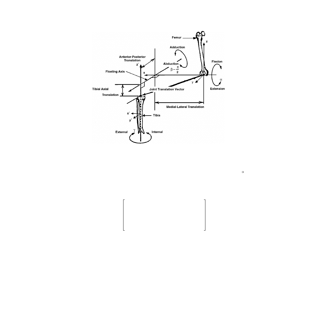
The tibio-femoral joint coordinate system introduced by Grood and Suntay was used to define the
rotation and translation vectors that describe the three-dimensional tibio-femoral motions.
61
This joint
coordinate system is shown in
and consists of an axis (x-axis) that is fixed on the femur (î is a
unit vector parallel to the x-axis), an axis (z
′
-axis) that is fixed on the tibia (k
′
ˆ parallel to the z
′
-axis),
and a floating axis perpendicular to these two fixed axes (ê
2
is a unit vector parallel to the floating axis).
The three components of the rotation vector include flexion-extension, tibial internal-external, and varus-
valgus rotations. Flexion-extension rotations,
α
, occur around the femoral fixed axis; internal-external
tibial rotations,
γ
, occur about the tibial fixed axis; and varus-valgus rotations,
β
, (ad-abduction) occur
about the floating axis. Using this joint coordinate system, the rotation vector, , describing the orien-
tation of the tibial coordinate system with respect to the femoral coordinate system is written as:
= –
α
î
–
β
ê
2
–
γ
ˆk
′′′′
(1.1)
This rotation vector can be transformed to the femoral coordinate system, then differentiated with respect
to time to yield the angular velocity and angular acceleration vectors of the tibia with respect to the femur.
In this analysis, it is assumed that the femur is fixed while the tibia is moving. The locations of the
attachment points of the ligamentous structures as well as other bony landmarks are specified on each
bone and expressed with respect to a local bony coordinate system. The distances between the tibial and
femoral attachment points of the ligamentous structures are calculated in order to determine how the
lengths of the ligaments change during motion. Analysis includes expressing the coordinates of each
attachment point with respect to one bony coordinate system: the tibia or the femur. This is accomplished
by establishing the transformation between the two coordinate systems. The six parameters (three rota-
tions and three translations) describing tibio-femoral motions were used to determine this transformation
as follows:
θ
θθθθ
© 2001 by CRC Press LLC
→
R
=
→
R
o
+ [R]
r
→
(1.2)
where
→
r
describes the position vector of a point with respect to the tibial coordinate system, and
describes the position vector of the same point with respect to the femoral coordinate system. The vector
R
o
→
is the position vector which locates the origin of the tibial coordinate system with respect to the
femoral coordinate system, and [R] is a (3
×
3) rotation matrix given by Grood and Suntay
61
as:
(1.3)
where
α
is the knee flexion angle,
γ
is the tibial external rotation angle, and
β
is (
π
/2± abduction); positive
sign indicates a right knee and negative sign indicates a left knee.
Contact and Geometric Compatibility Conditions
As indicated in the introductory section of this chapter, several methods have been reported in the
literature to provide three-dimensional mathematical representations of the articular surfaces of the
femur and tibia.
12,21,68,124
In this model, and for simplicity, geometric primitives are employed. The
coordinates of a sufficient number of points on the femoral condyles and tibial plateaus of several
cadaveric knee specimens were obtained from related studies.
67,136
A separate mathematical function was
determined as an approximate representation for each of the medial femoral condyle, the lateral femoral
condyle, the medial tibial plateau, and the lateral tibial plateau. The femoral articular surfaces were
approximated as parts of spheres, while the tibial plateaus were considered as planar surfaces as shown
FIGURE 1.1
Tibio-femoral joint coordinate system. (
Source
: Rahman, E.M. and Hefzy, M.S.,
JJBE: Med. Eng. Physics
,
20, 4, 276, 1998. With permission from Elsevier Science.)
R
R
[ ]
β
γ
cos
sin
β
γ
sin
sin
β
cos
α
γ
sin
cos
–
α
γ
cos
cos
α
β
sin
sin
α
β
γ
cos
cos
sin
–
α
β
γ
sin
cos
sin
–
α
γ
sin
sin
α
γ
cos
sin
–
α
β
sin
cos
α
β
γ
cos
cos
cos
–
α
β
γ
sin
cos
cos
–
=
© 2001 by CRC Press LLC
. The equations of the medial and lateral femoral spheres expressed in the femoral
coordinate system of axes were written as:
(1.4)
where values of parameters (r, h, k, and l) were obtained as 21, 23.75, 18.0, 12.0 mm and 20.0, 23.0, 16.0,
11.5 mm for the medial and lateral spheres, respectively. The equations of the medial and lateral tibial
planes expressed in the tibial coordinate system of axes were written as:
g(x
′
, y
′
) = my
′
+ c
(1.5)
where values of parameters (m, c) were obtained as 0.358, 213 mm and –0.341, 212.9 mm for the medial
and lateral planes, respectively.
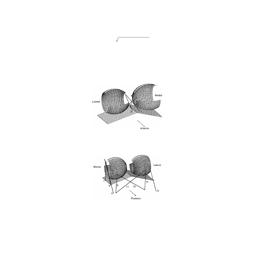
FIGURE 1.2
Three-dimensional model of the knee joint showing the anterior and posterior cruciate ligaments.
(1) AAC, Anterior fibers of the anterior cruciate; (2) PAC, posterior fibers of the anterior cruciate; (3) APC, anterior
fibers of the posterior cruciate; (4) PPC, posterior fibers of the posterior cruciate.
FIGURE 1.3
Three-dimensional model of the knee joint showing the collateral ligaments and the capsular struc-
tures. (5) AMC, anterior fibers of the medial collateral; (6) OMC, oblique fibers of the medial collateral; (7) DMC,
deep fibers of the medial collateral; (8) LCL, lateral collateral; (9) MCAP, medial fibers of the posterior capsule; (10)
LCAP, lateral fibers of the posterior capsule; (11) OPL, oblique popliteal ligament; (12) APL, arcuate popliteal
ligament. (
Source
: Rahman, E.M. and Hefzy, M.S.,
JJBE: Med. Eng. Physics
, 20, 4, 276, 1998. With permission from
Elsevier Science.)
f x y
,
(
)
r
2
x
h
–
(
)
2
–
y
k
–
(
)
2
–
–
1
+
=

© 2001 by CRC Press LLC
This model accomodates two situations: a two-point contact and a single-point contact. Initially, a
two-point contact situation is assumed with the femur and tibia in contact on both medial and lateral
sides. In the calculations, if one contact force becomes negative, then the two bones within its compart-
ment are assumed to be separated, and the single-point contact situation is introduced, thus maintaining
contact in the other compartment.
The contact condition requires that the position vectors of each contact point in the femoral and the
tibial coordinate systems,
→
R
c
and
→
r
c
, respectively, satisfy Eq. (1.2) as follows:
→
R
c
= R
0
+ [R]r
c
→
(1.6)
where
(1.6.a)
→
r
c
= x
c
′ î′ˆ + y
c
′ ˆj
′
ˆ
+ z
c
′
ˆk
′
ˆ
(1.6.b)
where x
c
, y
c
, z
c
and x
c
′, y
c
′, z
c
′ are the coordinates of the contact points in the femoral and tibial systems,
respectively. Since contact occurs at points identifiable in both the femoral and tibial articulating surfaces,
we can write at each contact point:
z
c
= f(x
c
, y
c
)
(7.a)
z
c
′ = g(x
c
′, y
c
′)
(7.b)
where f(x
c
, y
c
) and g(x
c
′, y
c
′) are given by Eqs. (1.4) and (1.5), respectively. Eq. (1.6) can thus be rewritten
as three scalar equations:
x
c
= x
0
+ R
11
x
c
′ + R
12
y
c
′ + R
13
g(x
c
′, y
c
′)
(1.8.a)
y
c
= y
0
+ R
21
x
c
′ + R
22
y
c
′ + R
23
g(x
c
′, y
c
′)
(1.8.b)
f(x
c
, y
c
) = z
0
+ R
31
x
c
′ + R
32
y
c
′ + R
33
g(x
c
′, y
c
′)
(1.8.c)
where R
ij
is the ijth component of the rotational transformation matrix (R). Eqs. (1.8a) through (1.8c)
constitute a mathematical definition for a contact point. Satisfying these equations at some given point
will ensure that it is a contact point. Thus, in the two-point contact version of the model, Eqs. (1.8a)
through (1.8c) generate six scalar equations which represent the contact conditions. In the one-point
contact version of the model, Eqs. (1.8a) through (1.8c) produce three scalar equations which represent
the contact conditions.
The geometric condition of compatibility of rigid bodies requires that a single tangent plane exists to
both femoral and tibial surfaces at each contact point. This condition also implies that the normals to
the femoral and tibial surfaces at each contact point are always colinear, and their cross product must
vanish.
In order to express the geometric compatibility condition in a mathematical form, the position vector
of the contact point in the femoral coordinate system (Eq. 1.6.a) is differentiated with respect to the local
(x and y) coordinates to obtain two tangent vectors along these local directions. Cross product of these
two tangent vectors is then employed to determine the unit vector normal to the femoral surface,
, at
the contact point. Using Eq. (1.7a), this unit vector is expressed in the femoral coordinate system as:
R
c
x
c
iˆ
y
c
jˆ
z
c
kˆ
+
+
=
nˆ
f
© 2001 by CRC Press LLC
(1.9)
A similar analysis is performed to obtain the unit vector normal to the tibial surface, ˆn
t
′′′′, at the contact
point. Using Eq. (1.7b), this unit vector is expressed in the tibial coordinate system as:
(1.10)
Applying the rotational transformation matrix to Eq. (1.10) yields the unit normal vector to the tibial
surface, ˆn
t
, expressed in the femoral coordinate system as:
(1.11)
Since the unit vectors normal to the surfaces of the femur and tibia are colinear, they are equal:
ˆn
f
= ˆn
t
(1.12)
This vectorial equation is rewritten in a scalar form as:
(1.13a)
(1.13b)
Eqs. (1.13a) and (1.13b) represent the geometric compatibility conditions at each contact point. Thus,
for each contact point, two independent scalar equations are written generating four scalar equations to
represent the geometric compatibility conditions in the two-point contact situation and two scalar
equations to represent the geometric compatibility conditions in the one-point contact situation.
Ligamentous Forces
In this analysis, external loads are applied, and ligamentous and contact forces are then determined. The
model includes 12 nonlinear spring elements that represent the different ligamentous structures and the
capsular tissue posterior to the knee joint. Four elements represent the respective anterior and posterior
fiber bundles of the anterior cruciate ligament (ACL) and the posterior cruciate ligament (PCL); three
elements represent the anterior, deep, and oblique fiber bundles of the medial collateral ligament (MCL);
one element represents the lateral collateral ligament (LCL); and four elements represent the medial,
lateral, and oblique fiber bundles of the posterior part of the capsule (CAP). These twelve elements are
shown in
. The coordinates of the femoral and tibial insertion sites of the different
ˆ
ˆ
ˆ
ˆ
@
,
,
n
j
k
f
=
∂
∂
+ ∂
∂
−
+ ∂
∂
+ ∂
∂
( )
=
(
)
(
)
(
)
f
x
i
f
y
f
x
f
y
x, y
x , y
x y
x y
c
c
c
c
c
c
1
2
2
ˆ
ˆ
ˆ
ˆ
@
,
,
′ =
∂
∂ ′
′ + ∂
∂ ′
′ − ′
+ ∂
∂ ′
+ ∂
∂ ′
′ ′
(
)
= ′ ′
(
)
′ ′
(
)
′ ′
(
)
n
j
k
t
g
x
i
g
y
g
x
g
y
x , y
x , y
x y
x y
c
c
c
c
c
c
1
2
2
ˆ
ˆ
ˆ
ˆ
n
i
j
k
t
=
′ +
′ −
′
(
)
+
′ +
′ −
′
(
)
+
′ +
′ −
′
(
)
′
′
′
′
′
′
′
′
′
R n
R n
R n
R n
R n
R n
R n
R n
R n
11
tx
12
ty
13
tz
21
tx
22
ty
23
tz
31
tx
32
ty
33
tz
n
R n
R n
R n
x, y
x , y
and
x , y
x , y
fx
11
tx
12
ty
13
tz
c
c
c
c
=
′ +
′ −
′
(
)
( )
=
(
)
′ ′
(
)
= ′ ′
(
)
′
′
′
@
n
R n
R n
R n
x, y
x , y
and
x , y
x , y
fy
21
tx
22
ty
23
tz
c
c
c
c
=
′ +
′ −
′
(
)
( )
=
(
)
′ ′
(
)
= ′ ′
(
)
′
′
′
@

© 2001 by CRC Press LLC
ligamentous structures were specified according to the data available in the literature.
20,36
These coordi-
nates are listed in
In the present analysis, ligament wrapping around bone was not taken into consideration. The spring
elements representing the ligamentous structures were thus assumed to be line elements extending from
the femoral origin to the tibial insertion. These elements were assumed to carry load only when they are
in tension, that is, when their length is larger than their slack, unstrained length, L
o
. Ligaments exhibit
a region of nonlinear force-elongation relationship, the “toe” region, in the initial stage of ligament strain,
then a linear force-elongation relationship in later stages.
134
A two-piece force-elongation relationship
was thus used to evaluate the magnitudes of the ligamentous forces.
21-23,118,129
This relationship is com-
posed of two regions: a linear region and a parabolic region. The magnitude of the force in the jth
ligamentous element is thus expressed as:
(1.14)
where K1
j
and K2
j
are the stiffness coefficients of the jth spring element for the parabolic and linear
regions, respectively, and L
j
and L
oj
are its current and slack lengths, respectively. The strain in the jth
ligamentous element,
ε
j
, is given by
(1.15)
and the linear range threshold is specified as
ε
1
= 0.03.
Values of the stiffness coefficients of the spring elements used to model the different ligamentous
structures were estimated according to the data available in the literature
21,23,30,93-96,109,118,129,130,133
and are
listed in
. The slack length of each spring element is obtained by assuming an extension ratio
e
j
at full extension and using the following relation:
TABLE 1.1
Local Attachment Coordinates of the Ligamentous Structures of the Present Model
Femur
Tibia
Ligament
x (mm)
y (mm)
z (mm)
x
′ (mm)
y
′ (mm)
z
′ (mm)
ACL, ant. fibers
7.25
–15.6
21.25
–7.0
5.0
211.25
ACL, post. fibers
7.25
–20.3
19.55
2.0
2.0
212.25
PCL, ant. fibers
–4.75
–11.2
14.05
5.0
–30.0
206.25
PCL, post. fibers
–4.75
–23.2
15.65
–5.0
–30.0
206.25
MCL, ant. fibers
–34.75
–1.0
26.25
–20.0
4.0
171.25
MCL, oblique fibers
–34.75
–8.0
24.25
–35.0
–30.0
199.25
MCL, deep fibers
–34.75
–5.0
21.25
–35.0
0.0
199.25
LCL
35.25
–15.0
21.25
45.0
–25.0
176.25
Post. capsule, med.
–24.75
–38.0
6.25
–25.0
–25.0
181.25
Post. capsule, lat.
25.25
–35.5
8.25
25.0
–25.0
181.25
Post. capsule, oblique popliteal ligament
25.25
–35.5
8.25
–25.0
–25.0
181.25
Post. capsule, arcuate popliteal ligament
–24.75
–38.0
6.25
25.0
–25.0
181.25
ACL: Anterior Cruciate Ligament.
PCL: Posterior Cruciate Ligament.
MCL: Medial Collateral Ligament.
LCL: Lateral Collateral Ligament.
(Source: Rahman, E.M. and Hefzy, M.S., JJBE: Med. Eng. Physics, 20, 4, 276, 1998. With permission from
Elsevier Science.)
F
0
;
0
K1 L
L
; 0
2
K2 L
1
L
;
2
j
j
j
j
oj
2
j
1
j
j
1
oj
2
j
1
=
≤
−
(
)
≤
≤
− +
(
)
(
)
≥
ε
ε
ε
ε
ε
ε
ε
j
j
oj
oj
L
L
L
=
−

© 2001 by CRC Press LLC
(1.16)
to evaluate the spring element’s slack length, L
oj
, from its length at full extension (which can be calculated
using the coordinates of the attachment points). The values of the extension ratios were specified
according to the data available in the literature
20,60
and are listed in
Contact Forces
As the tibia moves with respect to the femur, the contact points also move in the respective medial and
lateral compartments. Contact forces are induced at one or both contact points. These forces are applied
TABLE 1.2
Stiffness Coefficients of the Spring Elements Representing the
Ligamentous Structures of the Present Model
Ligament
K1 (N/mm
2
)
K2 (N/mm
2
)
ACL, ant. fibers
83.15
22.48
ACL, post. fibers
83.15
26.27
PCL, ant. fibers
125.00
31.26
PCL, post. fibers
60.00
19.29
MCL, ant. fibers
91.25
10.00
MCL, oblique fibers
27.86
5.00
MCL, deep fibers
21.07
5.00
LCL
72.22
10.00
Post. capsule, med.
52.59
12.00
Post. capsule, lat.
54.62
12.00
Post. Capsule, oblique popliteal ligament
21.42
3.00
Post. Capsule, arcuate popliteal ligament
20.82
3.00
ACL: Anterior Cruciate Ligament.
PCL: Posterior Cruciate Ligament.
MCL: Medial Collateral Ligament.
LCL: Lateral Collateral Ligament.
(Source: Rahman, E.M. and Hefzy, M.S., JJBE: Med. Eng. Physics, 20, 4, 276,
1998. With permission from Elsevier Science.)
TABLE 1.3
Extension Ratios at Full Extension of the
Ligamentous Structures of the Present Model
Ligament
e
ACL, ant. fibers
1.000
ACL, post. fibers
1.051
PCL, ant. fibers
1.004
PCL, post. fibers
1.050
MCL, ant. fibers
0.940
MCL, oblique fibers
1.031
MCL, deep fibers
1.049
LCL
1.050
Post. capsule, med.
1.080
Post. capsule, lat.
1.080
Post. capsule, oblique popliteal ligament
1.080
Post. capsule, arcuate popliteal ligament
1.070
ACL: Anterior Cruciate Ligament.
PCL: Posterior Cruciate Ligament.
MCL: Medial Collateral Ligament.
LCL: Lateral Collateral Ligament.
(Source: Rahman, E.M. and Hefzy, M.S., JJBE: Med. Eng.
Physics, 20, 4, 276, 1998. With permission from Elsevier
Science.)
ε
j
j
at full extension
oj
L
L
=

© 2001 by CRC Press LLC
normal to the articular surface. Thus, the contact force applied to the tibia is expressed as:
=
where
N
i
is the magnitude of the contact force, and ˆn
i
is the unit vector normal to the tibial surface at the
contact point, expressed in the femoral coordinate system. In the two-point contact situation, i = 1, 2
and in the single-point contact situation, i = 1.
Equations of Motion
The equations governing the three-dimensional motion of the tibia with respect to the femur are the
second order differential Newton’s and Euler’s equations of motion. Newton’s equations are written in
a scalar form, with respect to the femoral fixed system of axes, as:
(1.17)
(1.18)
(1.19)
where m is the mass of the leg, ··x
o
, ··y
o
, and ··z
o
are the components of the linear acceleration of the center
of mass of the leg (in the fixed femoral coordinate system); W
x
, W
y
, and W
z
are the components of the
weight of the leg; and F
ex
, F
ey
, and F
ez
are the components of the external forcing pulse applied to the tibia.
Euler’s equations of motion are written with respect to the moving tibial system of axes which is the
tibial centroidal principal system of axes (x
′, y′ and z′). Thus, the angular velocity components
·
(
θ
x
′
,
·θ
y
′
,
θ
z
′
)
·
and angular acceleration components
··
(
θ
x
′
,
··
θ
y
′
,
··
θ
z
′
), in the Euler equations, are expressed with respect
to this principal system of axes as:
(1.20a)
(1.20b)
(1.20c)
(1.21a)
(1.21b)
(1.21c)
N
i
N n
i
i
ˆ
F
W
N
F = m x
ex
x
ix
i=
2
jx
j=1
12
o
+
+
+
∑ ∑
1
˙˙
F
W
N
F = m y
ey
y
iy
i=
2
jy
j=1
12
o
+
+
+
∑ ∑
1
˙˙
F
W
N
F = m z
ez
z
iz
i=
2
jz
j=1
12
o
+
+
+
∑ ∑
1
˙˙
˙
˙ sin cos
˙
cos cos
˙
sin sin
˙ sin
˙
cos
θ
α
β
γ α β
β
γ α γ
β
γ β
γ β γ
γ
′
= −
−
+
+
+
x
˙
˙ sin sin
˙
cos sin
˙
sin cos
˙ cos
˙ sin
θ
α
β
γ α β
β
γ α γ
β
γ β
γ β γ
γ
′
= −
−
−
+
+
y
˙
˙ cos
˙ sin
˙
θ
α
β αβ
β
′
= −
+
−
z
y
˙˙
˙˙ sin cos
˙˙
cos cos
˙˙
sin sin
˙
sin
˙
sin cos cos
˙
cos cos
˙ ˙
cos sin
˙
sin sin
sin
˙˙ cos
˙˙ ˙ cos
θ
α
β
γ α β
β
γ α γ
β
γ α β
γ α γ
β
β
γ
α β
β
γ
α β γ
β
γ
α γ
β
β
γ
β γ
γ
β γ
γ
′
= −
−
+
−
−
−
+
+
+
+
+
x
2
2
2
2
2
2
˙˙
˙˙ sin sin
˙˙
cos sin
˙˙
sin cos
˙
cos
˙
sin cos cos
˙
cos cos
˙ ˙
cos cos
˙ ˙ sin cos
˙˙ sin
˙˙ sin
˙˙ ˙ sin
θ
α
β
γ α β
β
γ α γ
β
γ α β
γ α γ
β
β
γ
α β
β
γ
α β γ
β
γ
α γ
β
γ β
γ
β γ
γ
β γ
γ
′
= −
−
−
−
−
−
+
−
−
+
+
y
2
2
2
2
2
2
˙˙
˙˙ cos
˙˙
sin
˙
sin
˙ ˙ sin
˙
– ˙˙
θ
α
β α β
β α γ
β
α β
β β γ γ
′
=
+
+
+
+
z
2
2
2
2

© 2001 by CRC Press LLC
Euler’s equations are written in a scalar form as:
(1.22)
(1.23)
(1.24)
where (
ΣM)
x
′
, (
ΣM)
y
′
, and (
ΣM)
z
′
are the sum of the moments of all forces acting on the tibia around
the x
′, y′, and z′ axis, respectively, and I
x
′x′
, I
y
′y′
, and I
z
′z′
are the principal moments of inertia of the leg
about this centroidal principal axis. The inertial parameters were estimated using the anthropometric
data available in the literature.
32,34,40,102,120
In this analysis, the mass of the leg was taken as m = 4.0 kg.
Also, the leg was assumed to be a right cylinder; mass moments of inertia were thus calculated as I
x
′x′
=
0.0672 kg m
2
, I
y
′y′
= 0.0672 kg m
2
, and I
z
′z′
= 0.005334 kg m
2
.
In the two point-contact situation, tibio-femoral motions are thus described in terms of six differential
equations of motion: Eqs. (1.17) through (1.19) and (1.22) through (1.24), and ten nonlinear algebraic
equations [six contact conditions: Eqs. (1.8a through 1.8c), and four geometric compatibility conditions:
Eqs. (1.13a) and (1.13b)]. In the one-point contact situation, the ten algebraic equations reduce to five:
three contact conditions and two geometric compatibility conditions. The governing system of equations
in the two-point contact version of the model thus consists of 16 equations in 16 unknowns: six motion
parameters (x
o
, y
o
, z
o
,
α, β, and γ); two contact forces (N
1
and N
2
); and eight contact parameters [(x
c1
,
y
c1
) and (x
c2
, y
c2
): the coordinates of the medial and lateral contact points in the femoral system of axes,
respectively, and (x
c1
′, y
c1
′) and (x
c2
′, y
c2
′): the coordinates of the medial and lateral contact points in the
tibial system of axes, respectively]. In the one-point contact version of the model, the governing system
of equations reduces to 11 equations in 11 unknowns.
1.3 Solution Algorithm
In this formulation, six second order ordinary differential equations (ODEs), Newton’s and Euler’s
equations of motion, are written to describe the general motion of the tibia with respect to the femur.
Two-point contact is initially assumed. At each contact point five nonlinear algebraic constraints are
written to satisfy the contact and compatibility conditions. Thus, this system of equations can be expressed
as:
→
F(y,
→
y,
→
y,
→
t) = 0
→
·
··
(1.25)
where
and
. This system has two parts: a differential part and an algebraic part. These
ODE systems are called differential-algebraic equations (DAEs). Numerical methods from the field of
ODEs have classically been employed to solve DAE systems.
24,53-56,105
The behavior of the numerical methods used to solve a DAE system depends on the DAE’s index.
While the existing DAE algorithms are robust enough to handle systems of index one, they encounter
difficulties in solving systems of higher indices. The index of a DAE system is the number of times the
algebraic constraints need to be differentiated in order to match the order of the differential part of the
system and at the same time be able to solve the DAE system for explicit expressions for each of the
components of the
·
vector
→
y.
55
In the present system, N
1
and N
2
, two independent variables in vector
→
y,
appear only in the differential equations of motion. In order to generate terms that include
·
N
1
and
N
2
,
·
which are components of vector
→
y,
·
the differential equations need to be differentiated once more
ΣM
I
I
I
y
y y
y
x x
z z
x
z
( )
=
+
−
(
)
′
′ ′
′
′ ′
′ ′
′
′
˙˙
˙ ˙
θ
θ θ
ΣM
I
I
I
y
y y
y
x x
z z
x
z
( )
=
+
−
(
)
′
′ ′
′
′ ′
′ ′
′
′
˙˙
˙ ˙
θ
θ θ
ΣM
I
I
I
z
z z
z
y y
x x
x
y
( )
=
+
−
(
)
′
′ ′
′
′ ′
′ ′
′
′
˙˙
˙ ˙
θ
θ θ
y
y
d
dt
˙
→
→
=
y
y
d
dt
˙
˙
→
=
→

© 2001 by CRC Press LLC
with respect to time. These equations are then transformed to third order differential equations. The
algebraic constraints are then differentiated thrice with respect to time in order to match the order of
the differential part of the system. Consequently, the present system of equations describing the dynamic
behavior of the knee joint has an index value of three.
To reduce the order of the system it is rewritten in an equivalent mathematical form which has the
same analytical solution but possesses a lower index. The second order time derivatives, accelerations in
the equations of motion, are transformed to first order time derivatives of velocity. The system is then
augmented with six more first order ordinary differential equations relating the joint motions to the
joint velocities. The differential part of the system is transformed to
v
x
= ·x
o
(1.26a)
v
y
= ·y
o
(1.26b)
v
z
= ·z
o
(1.26c)
ω
α
=
α
·
(1.26d)
ω
β
=
β
·
(1.26e)
ω
γ
=
γ ·
(1.26f )
(1.27a)
(1.27b)
(1.27c)
(1.27d)
(1.27e)
(1.27f )
Using Eqs. (1.26d) through (1.26f) into Eqs. (1.20) and (1.21),
ω
x
′
,
ω
x
′
,
ω
x
′
, ·
ω
x
′
, ·
ω
x
′
, and ·
ω
x
′
are expressed
as:
(1.28a)
(1.28b)
F
W
N
F
m v
ex
x
ix
i=1
jx
j=1
12
x
+
+
+
=
∑ ∑
2
˙
F
W
N
F
m v
ey
y
iy
i=1
jy
j=1
12
y
+
+
+
=
∑ ∑
2
˙
F
W
N
F
m v
ez
z
iz
i=1
jz
j=1
12
z
+
+
+
=
∑ ∑
2
˙
ΣM
I
I
I
x
xx
x
zz
yy
y
z
( )
=
+
−
(
)
′
′
′
′
′
′
′
˙
ω
ω ω
ΣM
I
I
I
y
yy
y
xx
zz
x
z
( )
=
+
−
(
)
′
′
′
′
′
′
˙
ω
ω ω
ΣM
I
I
I
z
zz
z
yy
xx
x
y
( )
=
+
−
(
)
′
′
′
′
′
′
˙
ω
ω ω
ω
ω
β
γ ω β
β
γ ω γ
β
γ ω
γ ω γ
γ
α
α
α
β
β
′
= −
−
+
+
+
x
sin cos
cos cos
sin sin
sin
cos
ω
ω
β
γ ω β
β
γ ω γ
β
γ ω
γ ω γ
γ
α
α
α
β
β
′
= −
−
−
−
+
y
sin sin
cos sin
sin cos
cos
sin

© 2001 by CRC Press LLC
(1.28c)
(1.29a)
(1.29b)
(1.29c)
The resulting system of equations contains twelve first order ordinary differential equations and ten
nonlinear algebraic constraints. It can be written as:
→
F(y,
→
y,
→
t)
·
= 0
→
(1.30)
where
is a vector of dimension (n = 22) containing the 22 independent variables, namely, {x
o
, y
o
, z
o
,
α, β, γ, v
x
, v
y
, v
z
,
ω
α
,
ω
β
,
ω
γ
, x
c1
, y
c1
, x
c2
, y
c2
, x
c1
′, y
c1
′, x
c2
′, y
c2
′, N
1
, and N
2
}. This is a DAE system of 22
equations to be solved in 22 unknowns. While it is mathematically equivalent to the original system, it
has an index of two. To generate
·
N
1
and
·
N
2
, the equations of motion (which are now of order one) are
to be differentiated once more bringing them to order two. The algebraic constraints are then differen-
tiated twice with respect to time so they can match the order of the differential part of the system.
Therefore, the new system of equations describing the dynamic behavior of the knee joint has an index
value of two.
To solve the DAE system, the algorithm divides the analysis time span into time steps of variable size,
h
i
, and time stations, t
i
. From time station t
n
, the algorithm takes a step forward on time of size h
n+1
to
evaluate and
and
at time station t
n+1
; that is,
t
n+1
= t
n
+ h
n +1
(1.31)
At each time station t
n+1
, components of
→
r
n+1
·
are approximated in terms of
→
y
n+1
and
at previous time
steps using an integration formula such as a backward differentiation formula (BDF) or a Runge-Kutta
(R-K) method. The most popular integration scheme is multistep BDF. This scheme yields:
(1.32)
where k is the order of the formula and (
α
i
, i = 0, k) are the coefficients of the BDF. These coefficients
are determined using generating polynomials such as those defined by Jackson and Sacks-Davis.
77
The
order of the BDF formula is equal to the number of steps over which it extrapolates the solution. At
every step h
n+1
, the order, k, and step size, h, used are dependent on the behavior of the solution.
ω
ω
β ω β
β ω
α
α
γ
′
= −
+
−
z
cos
sin
˙
˙ sin cos
˙
cos cos
˙
sin sin
sin
sin cos cos
cos cos
cos sin
sin sin
˙ sin
˙
cos
cos
ω
ω
β
γ ω β
β
γ ω γ
β
γ ω β
γ ω γ
β
β
γ
ω ω
β
γ
ω ω γ
β
γ
ω ω
β
γ ω
γ
ω γ
γ
ω ω
γ
α
α
α
α
α
α β
α β
α
γ
β
β
β
γ
′
= −
−
+
−
−
−
+
+
+
+
+
x
2
2
2
2
2
2
˙
˙
sin sin
˙
cos sin
˙
sin cos
cos
sin cos sin
cos sin
cos cos
sin cos
˙ cos
˙
sin
sin
ω
ω
β
γ ω β
β
γ ω γ
β
γ ω β
γ ω γ
β
β
γ
ω ω
β
γ
ω ω γ
β
γ
ω ω
β
γ ω
γ
ω γ
γ
ω ω
γ
α
α
α
α
α
α β
α β
α
γ
β
β
β
γ
′
= −
−
−
+
−
−
+
−
−
+
+
y
2
2
2
2
2
2
˙
˙ cos
˙
sin
sin
sin
˙
ω
ω
β ω β
β ω γ
β
ω ω
β ω γ ω
α
α
α
α β
α
γ
′
=
+
+
+
+
−
z
2
2
2
2
r
y
r
y
r˙
y
r
y
y
n
i
n
i
˙
→
→
+
+ −
=
∑
1
1
1
h
n+1
i=0
α
k
y

© 2001 by CRC Press LLC
Eq. (1.32) is hence used to eliminate
from the system of equations, and the DAE system defined in
Eq. (1.30) is transformed to the nonlinear algebraic system:
(1.33)
A
→
variation of the Newton-Raphson iteration technique is then used to solve the nonlinear system for
y
n+1
.
80
A solution for the resulting system is thus obtained using the differential form of the Newton-
Raphson method which includes evaluating iteratively {
} by solving the following system
of equations:
(1.34)
where
(1.35a)
and
(1.35b)
where
is defined by Eq. (1.30). After each iteration
is updated according to:
(1.36)
The iterations continue until
satisfies a pre-set convergence criterion. A local error test is then
carried out to check whether the solution satisfies user-defined error parameters. If the solution is
acceptable, the converged values of
→
y
N+1
and
are then used with values of and
and
at the
previous k time stations to evaluate
and
at t
n+2
and the algorithm continues marching on in time.
The stiffness matrix (K) used in step h
n+1
is carried on unchanged to step h
n+2
unless the algorithm fails
to complete step h
n+1
successfully. If the Newton-Raphson iterations fail to converge or the converged
solution fails to satisfy the user-defined error parameters, the algorithm goes back to t
n
and retakes the
step with an updated stiffness matrix, a smaller step size h, and/or a BDF of a different order.
The initial guess (i = 0) for
→
y
N+1
and
(required to begin the Newton-Raphson iterations) is pre-
dicted based on values of
at the previous k+1 time stations for a kth order integration formula. A
predictor polynomial, which interpolates
at the previous k+1 time stations, is used to extrapolate the
values of
at time station t
n+1
while its derivative is used to extrapolate the values of
at time station
t
n+1
. The extrapolation polynomial
24
can be written as:
(1.37)
where the recurrence formula of the divided differences is given by
r˙
y
F y
0
n 1
→
→
→
+
+
=
, t
n 1
∆∆
r
y
(i)
K y
y
R y
→
→
→
→
=
( )
,
,
t
t
∆
1
K y
F
y
F
y
→
→
→
→
→
= ∂
∂
+
∂
∂
→
→
,
˙
t
h
n+1,0, n+1
n+1,0, n+1
t
s
n+1
t
y
y
α
R y
F y
y
→
→
→
→
→
= −
( )
( )
,
,
,
˙
t
t
n+1, i-1
n+1, i-1
n+1
r
F
r
y
y
y
y
→
→
→
( )
( )
( )
=
+
n+1, i
n+1, i-1
i
∆∆
∆∆
y
→
( )
i
r˙
y
n+1
r
y
r˙
y
r
y
r˙
y
r˙
y
n+1
r
y
r
y
r
y
r˙
y
w
y
y
y
y
y
y
y
y
y
→
→
→
→
→
→
→
→
→
→
( )
=
+ −
(
)
+ −
(
)
−
(
)
+…+ −
(
)
−
(
)
… −
(
)
…
−
−
−
−
−
− +
−
−
n
n
n
n
n
n
n
n
n
n
n
n k
n
t
t
t
t
t
t
t
t
t
t
t
t
t
+
,
,
,
,
,
1
1
1
2
1
1
n 1
n 1
n k
,

© 2001 by CRC Press LLC
(1.38)
Using Eqs. (1.37) and (1.38),
and
are estimated by evaluating
(t) and
(t), respectively,
at (t = t
n+1
). This is called the predictor part of the algorithm while the solution of the nonlinear algebraic
system through Newton-Raphson iterations is called the corrector part of the algorithm. Algorithms
which use this approach are called predictor-corrector algorithms.
The initial values of
and
at t = t
o
(namely,
and
must be specified in order to completely
define this initial value problem. These initial conditions must be consistent, i.e., they must satisfy the
DAE system at time t = t
0
:
(1.39)
It is important to realize that DAE solvers are very sensitive to the initial conditions. A small inconsistency
in the initial conditions, especially for an index two DAE system, can cause the algorithm to diverge in
the first step.
24
DAE Solvers
Two major computer codes have been developed by the Lawrence Livermore National Laboratory to
integrate a DAE using the BDF: the Differential/Algebraic System Solver (DASSL) developed by Petzold
106
and the Livermore Solver for Ordinary Differential Equations: Implicit form (LSODI) developed by
Hindmarsh and Painter.
71
Both codes use error-controlled, variable-step, variable-order (integration
formula) predictor-corrector algorithms to integrate the DAE. Starting at time station (t
n
), the predictor
extrapolates the values of
and
at time station (t
n+1
) based on their values at earlier time stations using
a forward differentiation formula. Then the corrector utilizes a BDF of order ranging from one to five
to transform
→
F(y
n+1
,
→
y
n+1
,
→
t
n+1
) =
→
0 to the form
→
F(y
n+1
,
→
t
n+1
) =
→
0. The two codes differ in the BDF
formulas they use and in the step size, order selection, and error control strategies.
24
Both the load vector
and the stiffness matrix used in LSODI and DASSL are similar. In both codes, a solution for the resulting
system is then obtained using the differential form of the Newton-Raphson method which includes
solving Eq. (1.34) iteratively. After each corrector iteration a convergence test is carried; and after
convergence, a local error test is also carried.
We have used both LSODI and DASSL to obtain a solution for the present DAE system.
5-7
Some
instabilities were encountered when using the LSODI which is consistent with reports that DASSL is
more stable and robust.
24
Aside from having different error control strategies, the main difference between
the two codes is that while the LSODI uses a fixed coefficient implementation of the BDF formulas [Eq.
(1.32)], the DASSL uses a fixed leading coefficient implementation.
24
These two techniques allow the
multistep-fixed step size BDF formulas to accomodate multistep-variable step size applications. In the
fixed coefficient implementation, all coefficients of
→
y
n+1–i
are unchanged, even when different step sizes,
h
i
, are used. In the fixed leading coefficient implementation, only the first coefficient [that of
→
y
n+1
in Eq.
(1.32)] does not depend on the step size. We like to point out that Hindmarsh, one of the authors of
LSODI, indicated that the LSODI is essentially a stiff differential equation solver, and its use as a DAE
solver is only marginal (personal communication). In what follows, we briefly introduce the DASSL
software to the reader.
The DASSL computer code is a general purpose DAE solver designed to solve systems of indices zero
and one. It can also solve some classes of higher index DAEs including semi-explicit index two systems
such as the present DAE system.
y
y
y y
y
y y
y
y
y
y
→
→
→
→
→
→
→
→
→
→
→
=
…
=
…
−
…
−
−
−
−
− +
−
−
−
−
n
n
n
n
n k
n
n
n k
n
n
n k
n
n k
t
t
,
,
,
,
,
,
1
1
1
1
2
,
,
,
y
→
+
n 1
r˙
y
n+1
w
→
+
n 1
w
˙
→
+
n 1
r
y
r˙
y
r
y
0
r˙
y
0
)
F y
y
0
0
0
→
→
→
→
=
,
,
˙
t
0
r
y
r˙
y

© 2001 by CRC Press LLC
Input to the DASSL includes the initial time where the integration begins t = t
0
, the end of the
integration interval t = t
F
,
,
a relative error tolerance vector
→
ε
rel
and an absolute error tolerance
vector
→
εεεε
abs
. Each independent variable has a corresponding component in
→
ε
rel
and
→
ε
abs
. User supplied
subroutines evaluate the load vector
→
F(y,
→
y,
→
t)
·
and the stiffness matrix [K(y,
→
t)]. DASSL is called recur-
rently in a loop which updates t
F
until the analysis time span is covered.
The integration formula used by DASSL is a variable step size h variable order k fixed leading coefficient
α
s
version of the BDF. The order of the BDF can range from one to five.
24
At the first time station t
0
, the
code estimates the initial time step size h
1
in terms of t
F
, t
0
,
,
,
→
ε
rel
, and
→
ε
abs
. At each time station
t
n
, the predictor formula is used to evaluate
→
y
n+1,(0)
, then the corrector iterations are used to correct this
value. After each corrector iteration, a convergence test is carried out insuring that the weighted root
mean square norm of
→
∆∆∆∆y
(i)
is less than a pre-set convergence constant. The default norm used in DASSL
is a weighted root mean square norm, where the weights depend on the relative and absolute error
tolerance vectors and on the value of
at the beginning of the step. If the convergence test is not satisfied
after four iterations, the step is aborted. The algorithm goes back to station t
n
, calculates the stiffness
matrix, if it was not current, and repeats the step again. If it fails to converge again, the step size is reduced
by a factor of one quarter. If, after ten consecutive step size reductions, the code still fails to take the step,
or if at any time h becomes less than the minimum step size, h
min
, the code is aborted with a fatal error.
The minimum step size is either specified by the user or calculated by the code in terms of t
n
, t
F
, and
the computer roundoff error. If the code is aborted with a fatal error, the user needs to modify the
absolute and/or relative error vectors (error tolerance) and restart from the beginning.
If the convergence test is successful, a local error test is carried on the converged solution
→
y
n+1
. The
test amounts to requiring that the weighted root mean square norm of the difference between the
converged solution,
→
y
n+1
, and the predicted solution,
→
y
n+1,(0)
, be less than the user-defined error toler-
ances. If the test fails, the step is aborted and the algorithm goes back to t
n
and takes the step again.
Regardless of the success of the convergence test (or the local error test), an appropriate order of the
BDF and a new step size are calculated before a new step is taken (or before the same step is retaken).
The very first time step has to be taken with a BDF of order one (i.e., Euler’s method). Thereafter, and
for an initial number of subsequent steps (an initial phase), the code raises the order of the BDF, k, and
increases the step size, h. After that initial period, it begins to estimate the errors for different orders by
calculating the dominant terms in the remainder of a Taylor series expansion of the solution of order
k – 2, k – 1, k and k + 1, respectively. If the weighted root mean square norm of these quantities (error
estimates) decreases with the increase of the order, the order of the BDF, k, is increased by one and if
the weighted root mean square norm of the estimates increases with the increase of the order, the order
of the BDF, k, is decreased by one. A new step size is then calculated according to the estimate of the
local error in the last successful step. The smaller the local error estimate, the larger the next step size
will be (in comparison to the previous step). After a successful step, the change in the next step size never
exceeds a maximum of double or a minimum of half the previous step size. After an unsuccessful
attempted step, which as a result is retaken, the step size is decreased according to the local error estimate
in the last successful step. If more than one unsuccessful step has been attempted successively, then the
step size is decreased to 25% of its value.
After the local error test fails three times consecutively, the order of the BDF is reduced to one, since
a BDF of order one is the most stable fixed leading coefficient BDF at small step size. While trying to
satisfy the local error test, if h becomes smaller than h
min
the code is aborted with a fatal error; the user
must modify the error tolerance and restart from the beginning.
Load Vector and Stiffness Matrix
Expressions for the load vector, assuming contact on both the medial and lateral compartments, are
determined from Eq. (1.35b) as:
(1.40)
r
y
0
r˙
,
y
0
r
y
0
r˙
y
0
r
y
F
v
x
1
x
o
=
− ˙

© 2001 by CRC Press LLC
(1.41)
(1.42)
(1.43)
(1.44)
(1.45)
(1.46)
(1.47)
(1.48)
(1.49)
(1.50)
(1.51)
(1.52)
(1.53)
(1.54)
(1.55)
(1.56)
(1.57)
F
v
y
2
y
o
=
− ˙
F
v
z
3
z
o
=
− ˙
F
4
=
−
ω
α
α
˙
F
5
=
−
ω
β
β
˙
F
6
=
−
ω
γ
γ
˙
F
F
W
N
F
m v
7
ex
x
ix
i=1
jx
j=1
12
x
=
+
+
+
=
∑ ∑
2
˙
F
F
W
N
F
m v
8
ey
y
iy
i=1
jy
j=1
12
y
=
+
+
+
=
∑ ∑
2
˙
F
F
W
N
F
m v
9
ez
z
iz
i=1
jz
j=1
12
z
=
+
+
+
=
∑ ∑
2
˙
F
M
I
I
I
10
x
xx
x
zz
yy
y
z
=
( )
−
−
−
(
)
′
′
′
′
′
′
′
Σ
˙
ω
ω ω
F
M
I
I
I
11
y
yy
y
xx
zz
x
z
=
( )
−
−
−
(
)
′
′
′
′
′
′
′
Σ
˙
ω
ω ω
F
M
I
I
I
12
z
zz
z
yy
xx
x
y
=
( )
−
−
−
(
)
′
′
′
′
′
′
Σ
˙
ω
ω ω
F
x
x
R x
R y
R g x
y
13
c1
o
11
cl
12
cl
13 1
cl
cl
= −
+
+
′ +
′ +
′
′
(
)
,
F
y
y
R x
R y
R g x
y
14
c1
o
21
cl
22
cl
23 1
cl
cl
= −
+
+
′ +
′ +
′
′
(
)
,
F
f x
y
z
R x
R y
R g x
y
15
1
cl
cl
o
31
cl
32
cl
33 1
cl
cl
= −
(
)
+
+
′ +
′ +
′
′
(
)
,
,
F
x
x
R x
R y
R g x
y
16
c2
o
11
c2
12
c2
3
2
c2
c2
= −
+
+
′ +
′ +
′
′
(
)
1
,
F
y
y
R x
R y
R g x
y
1
c2
o
21
c2
22
c2
3
2
c2
c2
7
2
= −
+
+
′ +
′ +
′
′
(
)
,
F
f x
y
z
R x
R y
R g x
y
18
2
c2
c2
o
31
c2
32
c2
33
2
c2
c2
= −
(
)
+
+
′ +
′ +
′
′
(
)
,
,

© 2001 by CRC Press LLC
(1.58)
(1.59)
(1.60)
(1.61)
Eq. (1.35a) indicates that the stiffness matrix is the partial differential of each component of the load
vector with respect to each of the independent variables of the system. This leads to the development of
(22
× 22) and (17 × 17) stiffness matrices for the two-point contact and one-point contact situations,
respectively. Expressions for the elements forming these matrices are lengthy; they are listed in Reference 7.
1.4 Model Calculations
In a test situation, a sudden impact load was applied at the tibial center of mass with the knee straight.
This dynamic load was applied in a posterior direction perpendicular to the tibial mechanical axis. Impact
was simulated using sinusoidally decaying forcing pulses with different durations and different magni-
tudes. Each pulse is expressed as:
(1.62)
where A and t
o
are amplitude and pulse duration, respectively. Forcing pulses of this form can be simulated
experimentally
93
and have been used previously as typical representations of the dynamic load in head
impact analysis.
46
show the sinusoidally decaying forcing pulses of constant duration
and constant amplitude, respectively, that have been used in the present simulation. Sample results
showing the effects of varying pulse magnitude and pulse duration on knee flexion, varus-valgus rotations,
internal-external tibial rotations, linear and angular velocities of the tibia, ligamentous forces, and
magnitude and location of tibio-femoral contact forces are presented here.
In the analysis, the tibia was assumed to begin its motion from rest (v
x
= v
y
= v
z
=
ω
α
=
ω
β
=
ω
γ
= 0
at t = t
0
= 0 s) while the knee was fully extended (
α = 0°, β = 90°, γ = 0° at t = t
0
= 0 s). It was found
that the behavior of the system is very sensitive to the location of the initial contact points which required
using double precision while performing the computations. On the other hand, even a large error in the
initial values of the magnitude of the lateral and medial contact forces did not have an effect on the
system’s stability. This is because the behavior of a DAE system is very sensitive to unbalance only in its
F
n
R
n
R
n
R
n
x, y
x
y
and
x y
x
y
19
fx
11
tx
12
ty
13
tz
c1
c1
c1
c1
=
( )
−
′
( )
+
′
( )
−
′
( )
[
]
( )
=
(
)
′ ′
(
)
= ′
′
(
)
′
′
′
1
1
1
1
@
,
,
,
F
n
R
n
R
n
R
n
x, y
x
y
and
x y
x
y
20
fy
21
tx
22
ty
23
tz
c1
c1
c1
c1
=
( )
−
′
( )
+
′
( )
−
′
( )
[
]
( )
=
(
)
′ ′
(
)
= ′
′
(
)
′
′
′
1
1
1
1
@
,
,
,
F
n
R
n
R
n
R
n
x, y
x
y
and
x y
x
y
21
fx
11
tx
12
ty
13
tz
c2
c2
c2
c2
=
( )
−
′
( )
+
′
( )
−
′
( )
[
]
( )
=
(
)
′ ′
(
)
= ′
′
(
)
′
′
′
2
2
2
2
@
,
,
,
F
n
R
n
R
n
R
n
x, y
x
y
and
x y
x
y
22
fy
21
tx
22
ty
23
tz
c2
c2
c2
c2
=
( )
−
′
( )
+
′
( )
−
′
( )
[
]
( )
=
(
)
′ ′
(
)
= ′
′
(
)
′
′
′
2
2
2
2
@
,
,
,
F t
A e
t
t
e
-4.73
t
t
o
o
( )
=
2
sin
π
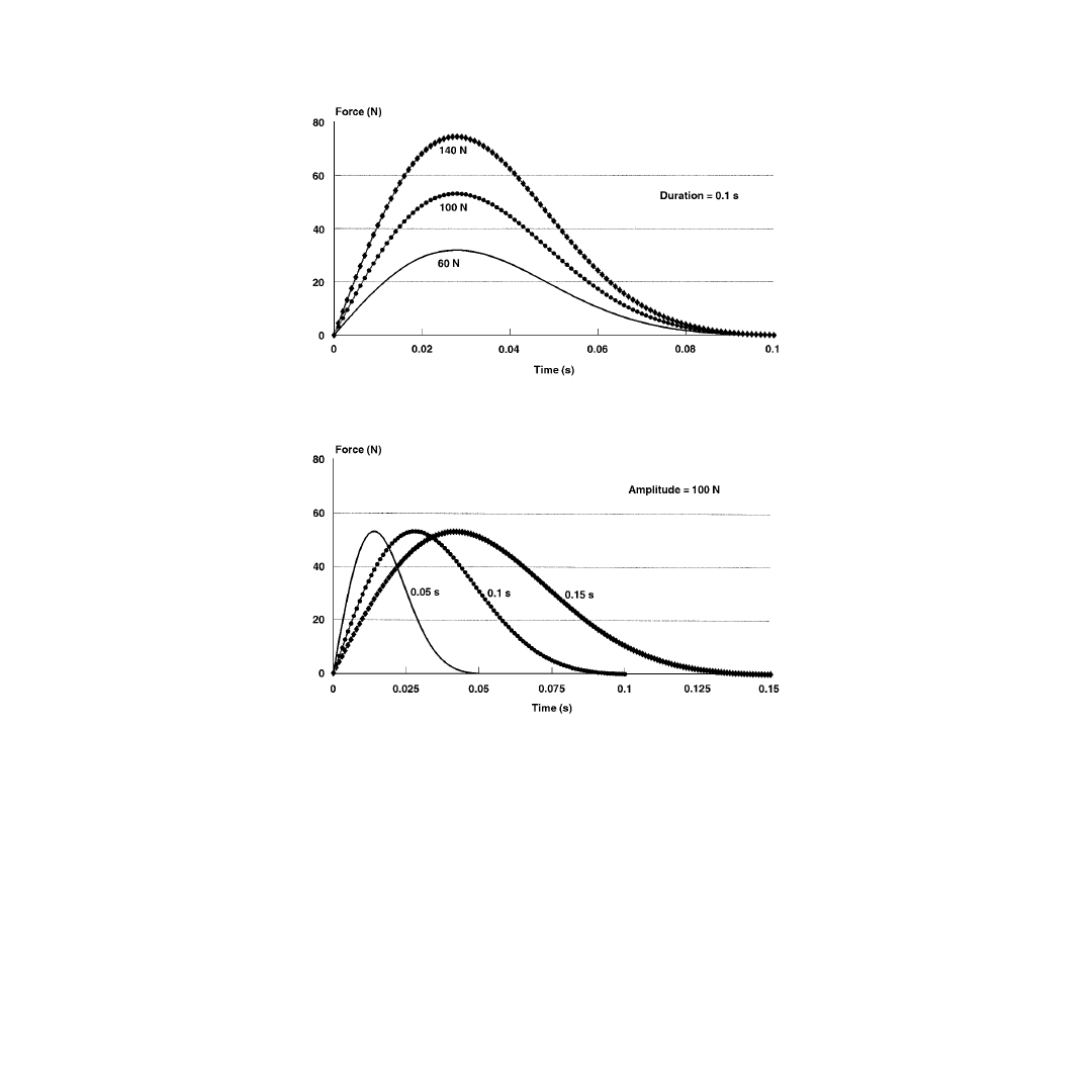
© 2001 by CRC Press LLC
algebraic part and not in its differential part. Since neither medial nor lateral contact forces appear in
the algebraic part of the DAE, the system is not sensitive to errors in their initial values.
The initial values of the x and y coordinates of the medial contact point in the local femoral and tibial
coordinate systems of axes were taken as x
c
= –16.72913866466 mm and y
c
= –18.540280082863 mm;
and x
c
′ = –16.980955 mm and y
c
′ = –12.8 mm, respectively. The initial values of the x and y coordinates
of the lateral contact point in the local femoral coordinate system were taken as x
c
= 16.50009371 mm
and y
c
= –16.00200022911 mm. The medial and lateral contact forces at t = t
0
= 0 s were assumed as
150.0 N and 130.0 N, respectively.
Using these assumed values, the coordinates of the tibial origin with respect to the femur at t = t
0
=
0 s were calculated using Eq. (1.88), thus satisfying the contact condition at the medial side. The initial
values of the x and y coordinates of the lateral contact point in the tibial coordinate system were then
calculated using Eq. (1.8) one more time, hence satisfying the contact condition at the lateral side. The
unbalance of the system (residual) at t = t
0
= 0 s is then determined using Eqs. (1.40) through (1.61).
An iterative procedure is then employed to determine the initial values of the 22 system variables that
minimize the initial residual.
FIGURE 1.4
Forcing pulses with different amplitudes and a constant duration of 0.1 s.
FIGURE 1.5
Forcing pulses with different durations and a constant amplitude of 100 N.
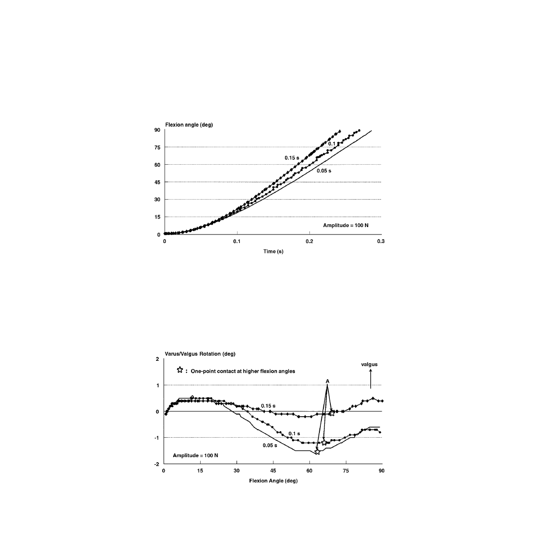
© 2001 by CRC Press LLC
shows how the knee flexion angle changes with time for a constant pulse amplitude of 100 N.
Increasing pulse duration caused the motion to become faster. This also occurred with increasing pulse
amplitude.
show how the varus-valgus rotation and the tibial axial rotation angles change
with knee flexion, respectively, for pulses with different duration and a constant amplitude of 100 N.
The one-point contact model was involved for joint positions with flexion angles larger than the flexion
angle at point (A), marked by a star, in each curve in
. For the rest of the figures presented
here, point A is not marked for conciseness.
shows that valgus rotation increased in the first 10° of knee flexion, decreased to zero between
25 and 45° of knee flexion, then varus rotation increased until the knee reached about 60° of flexion,
then decreased until 90° of knee flexion. The results indicate that the position at which the knee had
zero degrees of varus-valgus rotation changed from 25° of knee flexion to 45° of knee flexion when the
pulse duration was increased. Also,
shows that increasing the pulse duration caused a decrease
in the maximum amount of varus rotation. It was further found (not shown here) that increasing pulse
amplitude had the same effects as increasing pulse duration.
FIGURE 1.6
Flexion angle vs. time for different pulses of constant amplitude of 100 N.
FIGURE 1.7
Varus-valgus rotations vs. flexion angle.
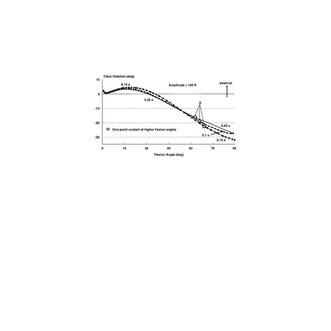
© 2001 by CRC Press LLC
shows that in the early stage of flexion, the tibia was externally rotated. This external rotation
increased until it reached a maximum when the knee was between 15 and 20° of knee flexion. At this
position, the knee started to go into internal rotation and reached a maximum at 90° of knee flexion.
The computer simulation indicates that increasing the pulse duration (and/or amplitude) produced an
increase in the magnitude of the maximum external and maximum internal rotation angles that occur
during knee flexion. Also, positions of the maximum external rotation angles were slightly affected by
the pulse amplitude and/or duration.
show the the femoral and tibial contact pathways, respectively, when a forcing pulse
of 100 N amplitude and 0.1 s duration was applied to the tibia.
shows that the medial and lateral
femoral contact points moved posteriorly and proximally as the knee was flexed from 0 to 90° of knee
flexion. A two-point contact condition was maintained until about 66° of knee flexion. From there on,
and until 90° of flexion, a one-point contact was predicted on the medial side.
shows that the
medial tibial contact point moved anteriorly, while the lateral tibial contact point moved posteriorly as
the knee was flexed from full extension. This motion is expected and can be thought of as a result of the
femur rotating externally over fixed plateaus which causes the medial tibial contact point to move
anteriorly and the lateral tibial contact point to move posteriorly. The analysis show that the position of
separation in the lateral compartment was slightly affected by the amplitude and/or duration of the
forcing pulses. However, the motion pattern of the medial and lateral femoral and tibial contact points
was independent of both pulse amplitude and pulse duration.
show how knee translational and rotational (angular) velocities changed with
knee flexion for pulses with different durations and a constant amplitude of 100 N.
shows that
the lateral shift velocity increased from zero at full extension to a maximum at about 15° of knee flexion,
then decreased, reaching zero around 30° of knee flexion. Henceforth, the medial shift velocity increased,
reaching a maximum at 90° of knee flexion.
shows that the posterior velocity increased from
zero at full extension to a maximum at about 50 to 60° of knee flexion, then decreased slightly as the
knee flexion increased.
shows that the knee flexion angular velocity increased monotonously
from zero at full extension, reaching a maximum at 90° of knee flexion.
shows that the valgus
velocity increased from zero at full extension to a maximum at about 5° of knee flexion, then decreased,
reaching zero around 10° of knee flexion. Then, the varus velocity increased, reaching a maximum
between 40 and 50° of knee flexion; henceforth, the velocity decreased reaching zero between 60 and 65°
of knee flexion. The valgus velocity increased again achieving a maximum around 80° of knee flexion.
shows that the internal rotation velocity increased from zero to a maximum at 2° of knee flexion
FIGURE 1.8
Tibial rotations vs. flexion angle.
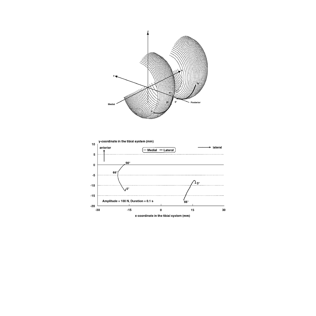
© 2001 by CRC Press LLC
and decreased to zero at 5° of knee flexion. Then, the external rotation velocity began to increase reaching
a maximum at around 8° of knee flexion and decreased, reaching zero around 20° of knee flexion. From
this point, the internal rotation velocity increased to a maximum between 45 and 60° of knee flexion
then decreased as the knee flexion increased.
The remaining results related to contact and ligamentous forces are shown for pulses of different
amplitudes and a constant duration of 0.1 s.
shows that the medial contact force decreased in
the first 15° of knee flexion, then increased until 60° of knee flexion, and then decreased until 90° of
knee flexion.
shows that the lateral contact force decreased from a maximum at full extension
until it reached zero when separation occurred in the lateral compartment. These two figures show that
increasing the pulse amplitude caused a decrease in the magnitude of the medial and lateral contact
forces; similar results were obtained when the pulse duration was increased while the pulse amplitude
was kept unchanged.
FIGURE 1.9
Femoral contact pathways. (
Source
: Rahman, E.M. and Hefzy, M.S.,
JJBE: Med. Eng. Physics
, 20, 4,
276, 1998. With permission from Elsevier Science.)
FIGURE 1.10
Tibial contact pathways. (
Source
: Rahman, E.M. and Hefzy, M.S.,
JJBE: Med. Eng. Physics
, 20, 4, 276,
1998. With permission from Elsevier Science.)
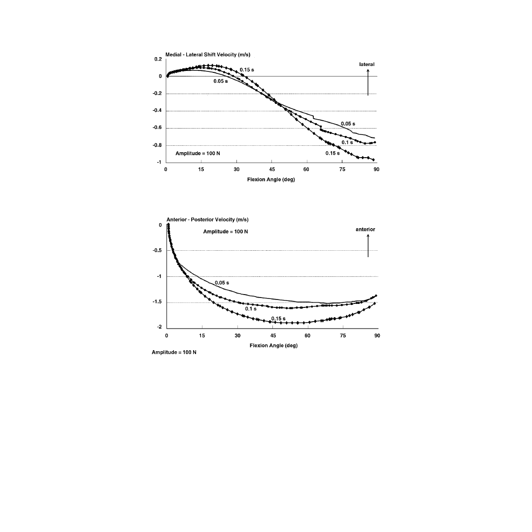
© 2001 by CRC Press LLC
show how the ligamentous forces changed with knee flexion.
show that in the first 20° of knee flexion, the tension in the anterior cruciate ligament is greatest in
its posterior fibers. As the flexion angle increased, this tension decreased while tension in the anterior
fibers increased and became dominant.
show that the anterior fibers of the posterior
cruciate ligament carried large forces after 45° of knee flexion while the posterior fibers were in tension
only in the first 10° of knee flexion.
show that within the medial collateral ligament, MCL, the deep fibers carried
more forces than the anterior fibers, which carried more forces than the oblique fibers which, in turn,
carried relatively very small forces. The maximum forces in the anterior and deep fibers occurred between
40 and 50° of knee flexion, while the maximum force in the oblique fibers occurred at approximately 5°
of knee flexion.
shows that the lateral collateral ligament sustained forces only in the first 45 to
60° of knee flexion, with a maximum value occurring near full extension.
FIGURE 1.11
Medial-lateral shift velocity vs. flexion angle.
FIGURE 1.12
Anterior-posterior velocity vs. flexion angle.
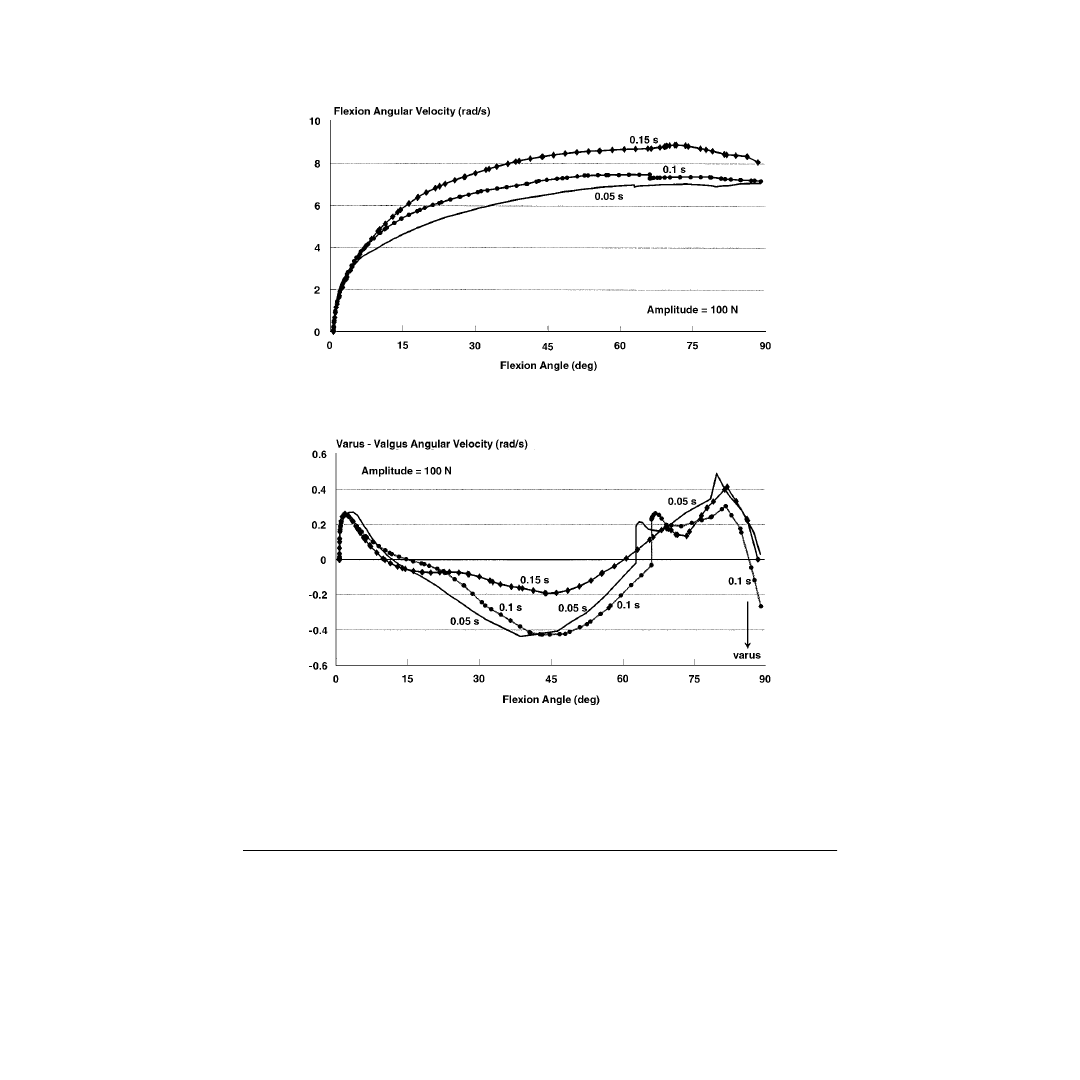
© 2001 by CRC Press LLC
The results show that the patterns of change in the ligamentous forces were not generally affected by
changing the characteristics of the applied pulsing loads. However, increasing pulse amplitude (and/or
duration) slightly affected the magnitude of the forces in the different ligamentous fibers.
1.5 Discussion
Review of the literature reveals that most of the published anatomical dynamic knee models are two-
dimensional
1-3,47-49,84,93-96
and that most of the existing three-dimensional anatomical knee models are
quasi-static in nature.
9,20-23,50,129,130
Quasi-static models determine forces and motion parameters by solving
the equilibrium equations, subject to appropriate constraints, at a specific knee position. The procedure
is then repeated at different positions to cover a range of knee motions. However, these quasi-static
models cannot predict the velocity or acceleration of the different segments forming the joint. Also, these
models are further limited in that they cannot determine the effects of the dynamic inertial loads
(which occur in many daily living activities) on joint kinematics and joint loads. In this chapter, a
FIGURE 1.13
Knee flexion angular velocity vs. flexion angle.
FIGURE 1.14
Varus-valgus angular velocity vs. flexion angle.
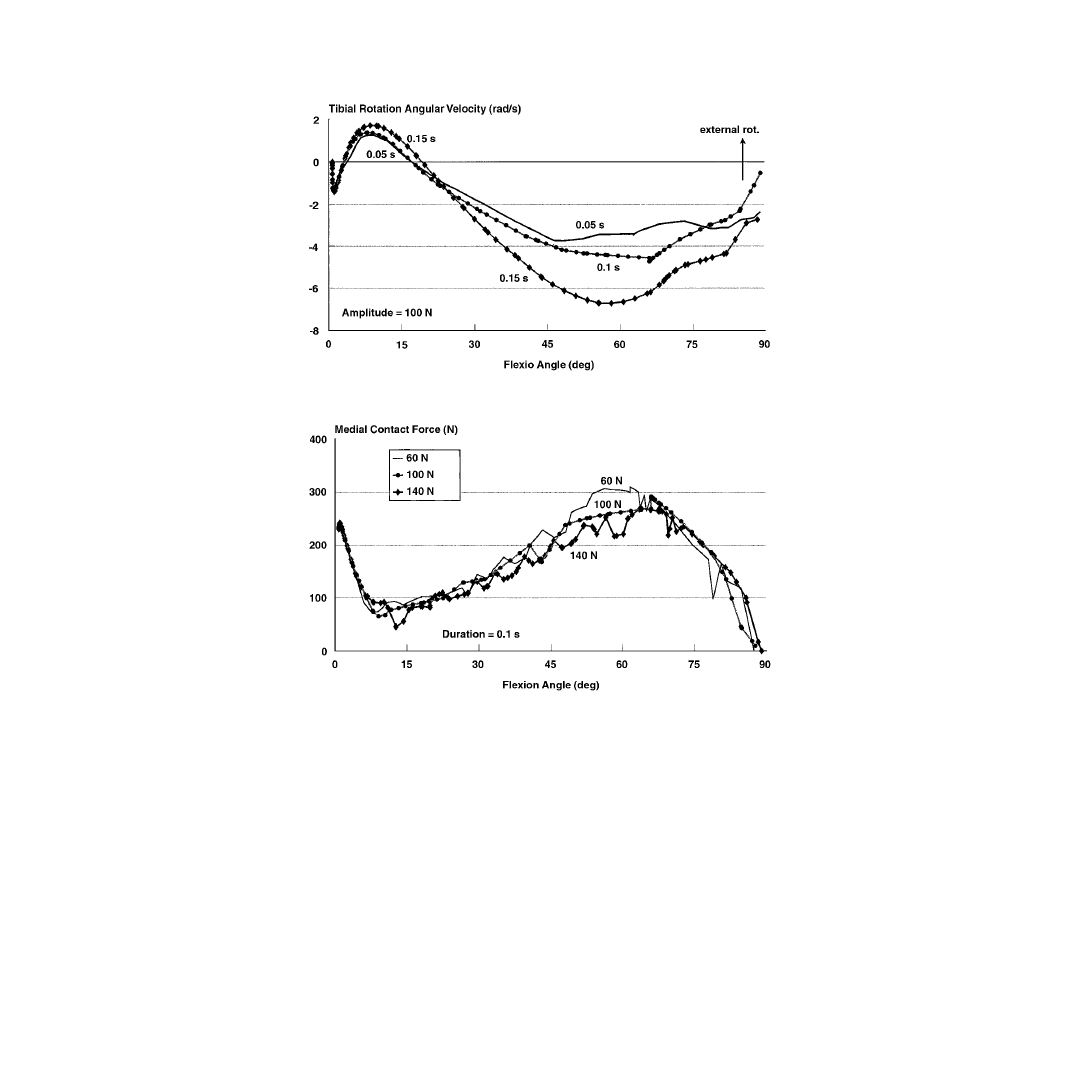
© 2001 by CRC Press LLC
three-dimensional dynamic anatomical model of the tibio-femoral joint that predicts its response under
sudden impact loads is presented.
The system of equations forming an anatomical quasi-static knee model is a system of nonlinear
algebraic equations. These equations are solved iteratively using a Newton-Raphson iteration tech-
nique,
20-23,129,130
discretized and solved using the finite element method
9
or rewritten as a potential energy
function that can be minimized using an optimization method such as the steepest descent optimization
technique.
50
On the other hand, the system of equations forming an anatomical dynamic model is a
system of differential algebraic equations (DAEs). Solving a DAE system is more difficult than solving
an algebraic system. Several techniques have been proposed to solve the DAE system that describes the
two-dimensional dynamic response of the knee joint.
1-3,47,84,93-96,118-119
These techniques were limited in
that they could not solve the DAE system that represents the three-dimensional situation. Using the
Differential/Algebraic System Solver software (DASSL) developed at the Lawrence Livermore National
Laboratory, the latter and more complex DAE system was solved, thus describing the three-dimensional
dynamic response of the knee joint. The integration scheme implemented in DASSL employs variable
order and variable size multistep backward differentiation formulas (BDFs).
FIGURE 1.15
Tibial rotation angular velocity vs. flexion angle.
FIGURE 1.16
Medial tibio-femoral contact force vs. flexion angle. (
Source
: Rahman, E.M. and Hefzy, M.S.,
JJBE:
Med. Eng. Physics
, 20, 4, 276, 1998. With permission from Elsevier Science.)
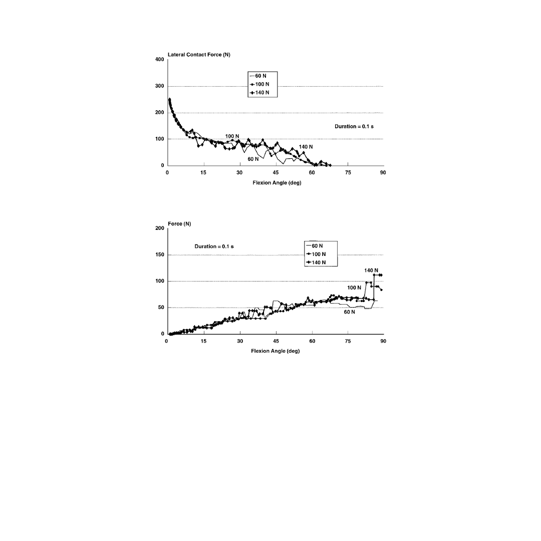
© 2001 by CRC Press LLC
It is hard to validate the present model predictions because of the limited experimental data available in
the literature that describe the dynamic behavior of the human knee joint. The dynamic response of the
joint must be described in terms of the loads exerted on the joint; the six components of the three-
dimensional motion of the tibia with respect to the femur; the deformations of the different components
forming the joint, including the ligaments, menisci and cartilage. Dortmans et al.
42
described the difficulties
associated with this task by stating that the dynamic behavior “... is much too complicated to deal with, due
to a lack of experimental techniques to quantify all parameters.” Keeping this in mind, model predictions
are discussed and, whenever appropriate, compared with the experimental data in the literature.
Varus-Valgus Rotation
Model predictions show that varus rotation occurred in association with internal tibial rotation while
the knee was flexed. These results are in agreement with van Kampen et al.
79
who reported that applying
internal torque to the tibia produced varus rotation. They are also in agreement with Essinger et al.’s
model calculations where varus rotations and internal tibial rotations were predicted with knee flexion.
50
FIGURE 1.17
Lateral tibio-femoral contact force vs. flexion angle. (
Source
: Rahman, E.M. and Hefzy, M.S.,
JJBE:
Med. Eng. Physics
, 20, 4, 276, 1998. With permission from Elsevier Science.)
FIGURE 1.18
Forces in the anterior fibers of the anterior cruciate ligament.
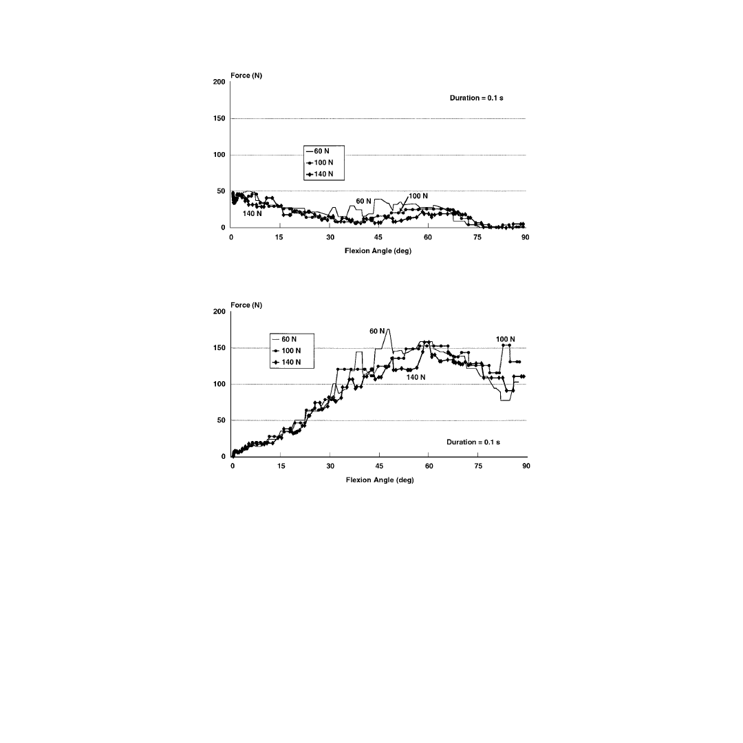
© 2001 by CRC Press LLC
Also, the results reported here are within the varus-valgus rotation’s envelope of passive knee motion
reported by Blankevoort et al.
19,21,23
and Mills and Hull.
91,92
The envelope of passive knee motion is the
region where the joint offers little resistance to motion. However, the model predictions are not in
agreement with the data reported by Blankevoort et al.
19,21,23
and Mills and Hull
91,92
where a valgus rotation
was coupled with and caused by the internal tibial rotation. This difference may be due to the omission
of the menisci in this model.
Mills and Hull
92
reported that the valgus rotation coupled with the internal tibial rotation is due to
the medial condyle’s ride over the medial meniscus. When an internal moment of 3 N-m was applied by
van Kampen et al.
79
to the tibia (significantly lower than the 20 N-m applied by Mills and Hull
91,92
which
did not force the ride of the femoral condyle over the medial meniscus), a varus rotation occurred with
knee flexion. Both the present model and Essinger et al.’s model
50
neglected the menisci and predicted
varus rotations associated with internal tibial rotation and knee flexion.
FIGURE 1.19
Forces in the posterior fibers of the anterior cruciate ligament.
FIGURE 1.20
Forces in the anterior fibers of the posterior cruciate ligament.
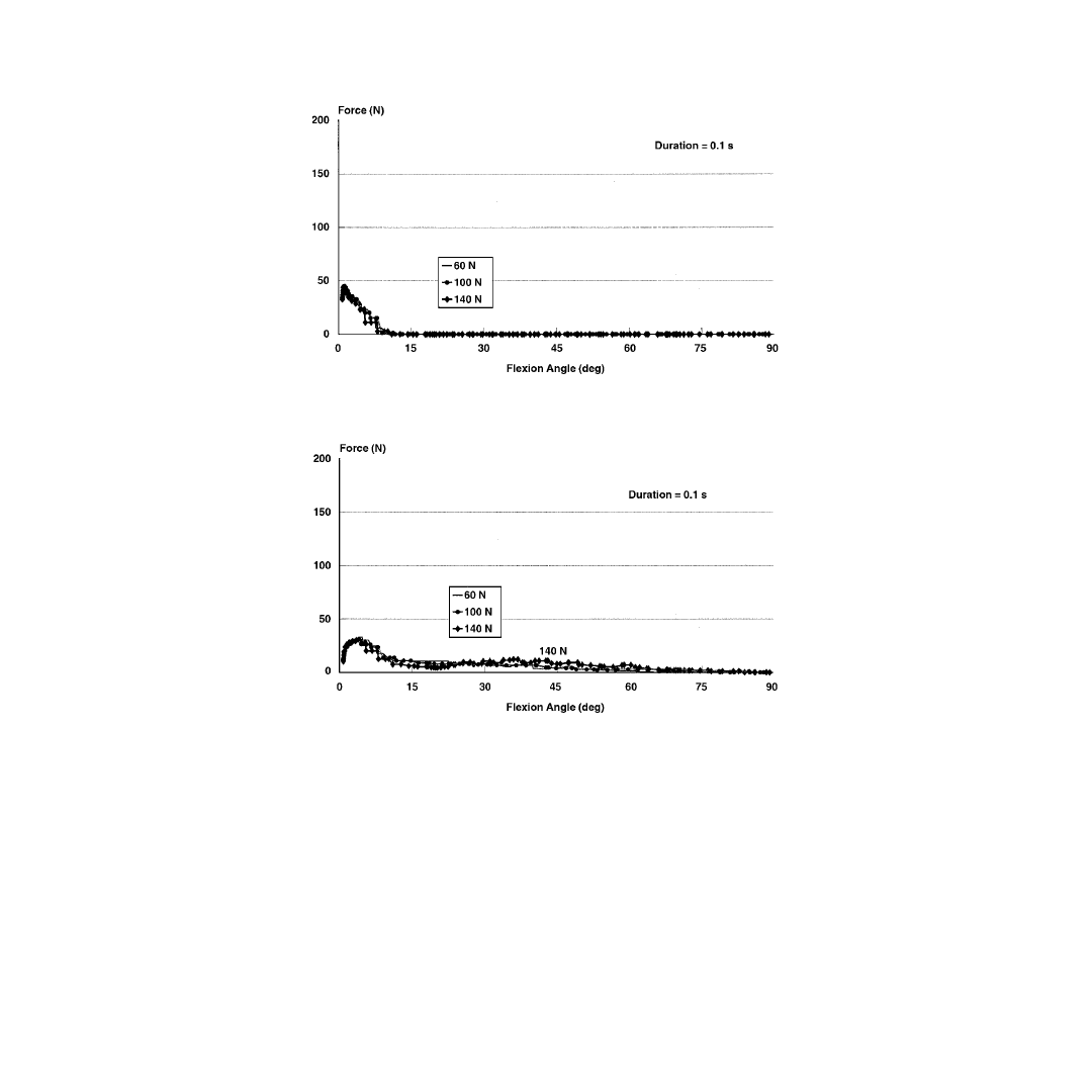
© 2001 by CRC Press LLC
Tibial Rotation
Model calculations show that as the knee was flexed from 15 to 90°, it underwent internal tibial rotation.
This rotation indicates that the tibia was subjected to internal moments caused by tension forces in the
lateral collateral ligament and/or the anterior fibers of both the anterior and posterior cruciate ligaments.
The predicted tibial rotations lay within the envelope of passive knee motion defined earlier.
19,21,23
Further,
these results are in agreement with those of Nigg et al.
103
who reported a mean internal tibial rotation
of 21.8° ± 8.4° during walking (that is, a range of 0 to 70° of knee flexion) and those of Essinger et al.
50
who reported an internal tibial rotation of 15° when the knee was flexed from full extension to 90° of
knee flexion.
These results indicate that external tibial rotation occurs with knee extension. However, this pattern
was not predicted by the model in the first 15° of knee flexion. This finding is important since it is in
agreement with the emerging thought of the need to re-evaluate the so-called screw-home mechanism
during dynamic motions. The “screw-home mechanism” is described as the external rotation of the tibia
with respect to the femur that occurs during the terminal stages of knee extension.
100
This mechanism
FIGURE 1.21
Forces in the posterior fibers of the posterior cruciate ligament.
FIGURE 1.22
Forces in the oblique fibers of the medial collateral ligament.
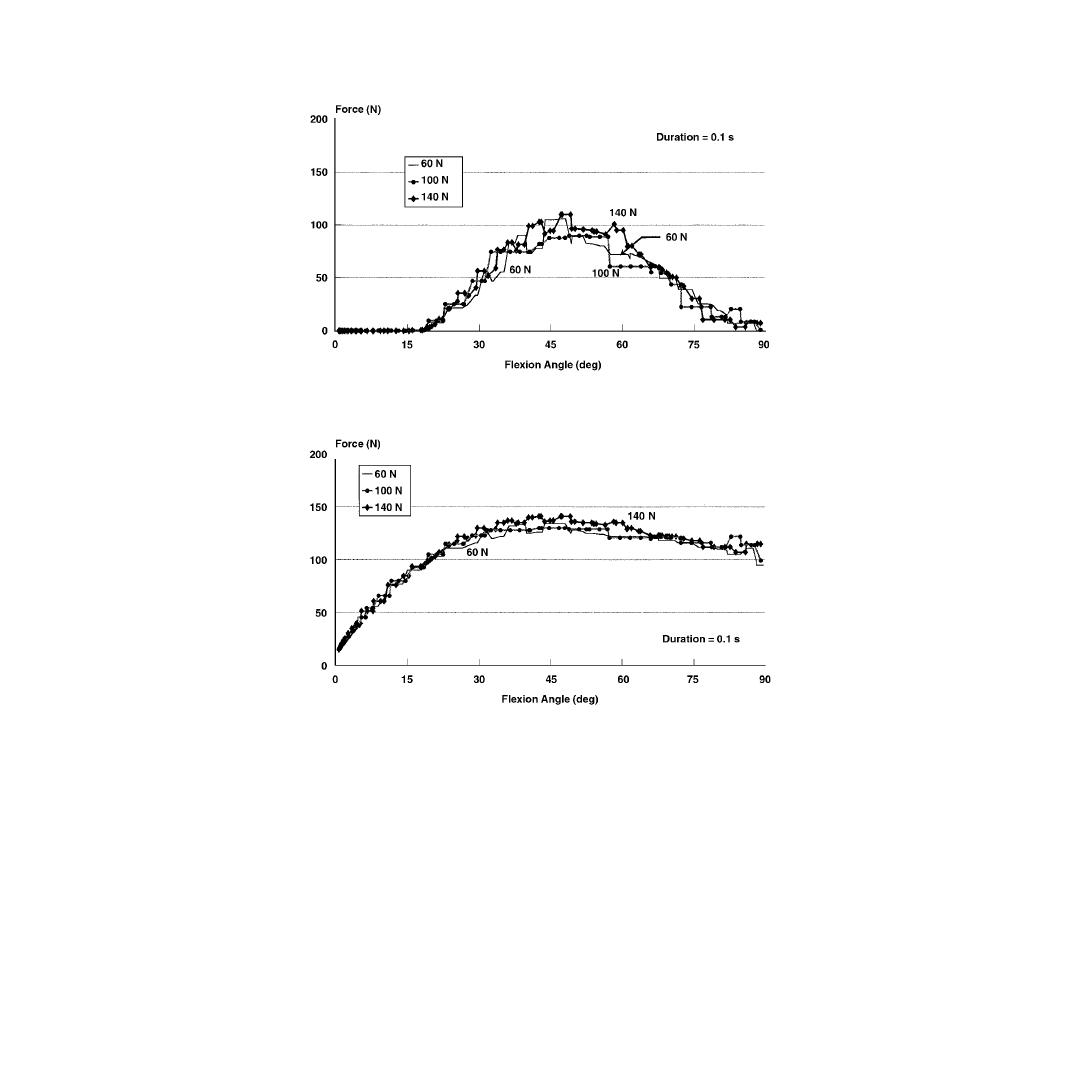
© 2001 by CRC Press LLC
was not predicted by this model since it was found that the tibia rotated internally as the knee was
extended from 15° to full extension. These results are in agreement with the recent data reported by
Blankevoort et al.
19
and Lafortune et al.
82
Lafortune et al. found that the tibia rotated internally with
respect to the femur in the terminal stage of knee extension. They stated that their results “appear to call
into question the accepted view that the tibia rotates externally relative to the femur in the later stages
of knee extension.” Blankevoort et al.
19
also reported that this screw-home mechanism was not present
when passive joint motion characteristics were determined.
Femoral and Tibial Contact Pathways
Model calculations show that the femoral contact points moved posteriorly and proximally with knee
flexion on both the medial and lateral femoral condyles over the whole range of knee flexion. There was
almost no medial-lateral shift on the femoral condyles. These results are in agreement with those obtained
using the two-dimensional four-bar linkage model
100,101
and those reported using two-dimensional ana-
tomical dynamic models.
1-3
These results are also in agreement with the data in the literature describing
FIGURE 1.23
Forces in the anterior fibers of the medial collateral ligament.
FIGURE 1.24
Forces in the deep fibers of the medial collateral ligament.
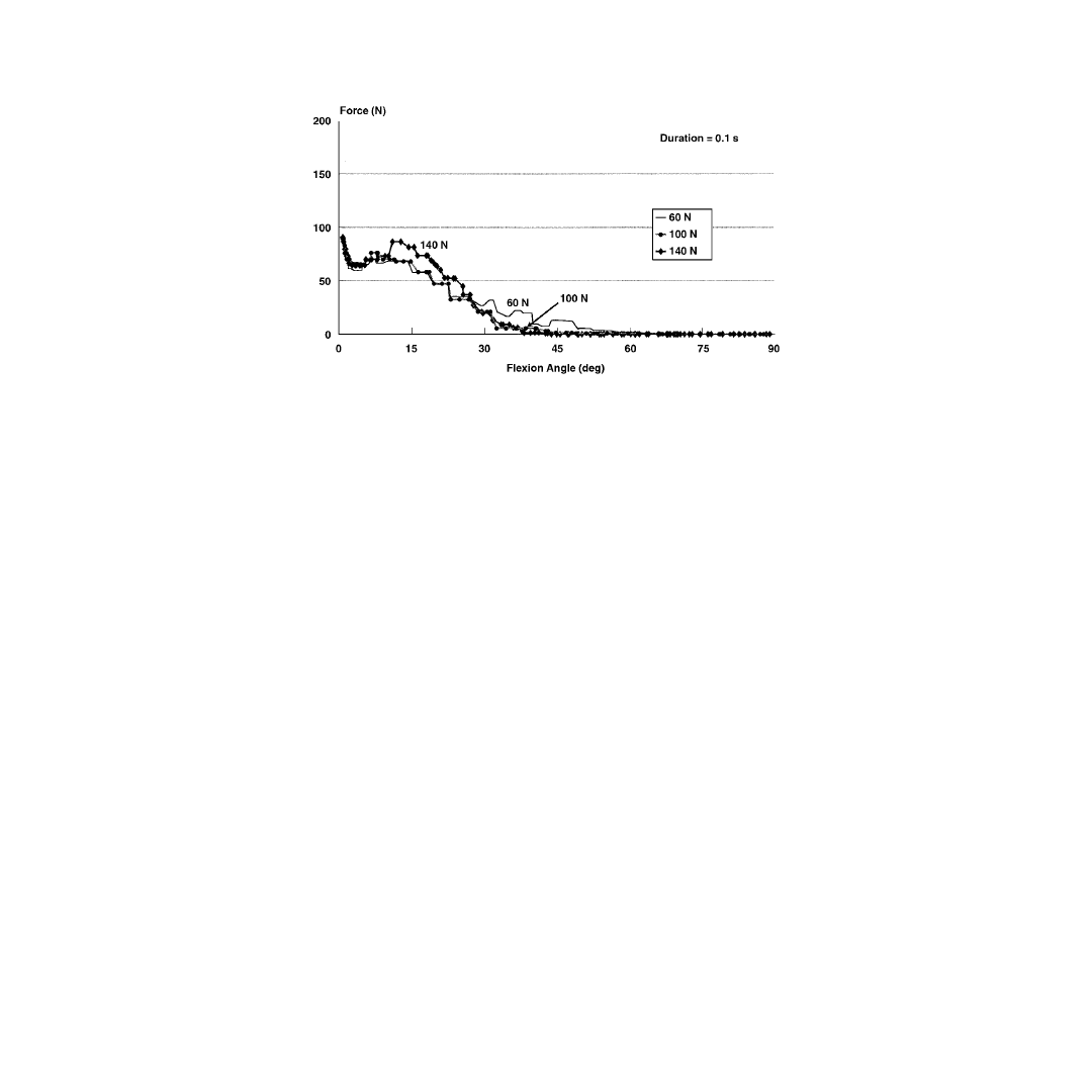
© 2001 by CRC Press LLC
the three-dimensional tibio-femoral contact characteristics where the tibio-femoral contact areas moved
posteriorly and proximally over the femoral condyles with knee flexion.
23,123
The medial tibial contact point was found to move anteriorly and the lateral tibial contact point to
move posteriorly when the knee was flexed beyond 15°. This is consistent with the predicted internal
tibial rotation pattern that occurred in this range of knee flexion. When separation occurred in the lateral
compartment, the medial contact point continued to move anteriorly to 90° of knee flexion as the internal
tibial rotation continued to be observed. Within the first 15° of knee flexion, the pattern describing the
pathways of the tibial contact points was reversed. The medial tibial contact point moved posteriorly,
while the lateral tibial contact point moved anteriorly. This pattern of motion was due to the external
tibial rotation sustained in this range of knee flexion.
Velocity of the Tibia
The posterior velocity of the tibia increased as it was flexed due to the application of the posterior load
which consisted of the forcing pulse and the leg’s weight. As the magnitude of the forcing pulse approached
zero and the component of the weight along the posterior axis decreased with knee flexion, the posterior
velocity leveled off to almost a constant magnitude for the remainder of the motion. The flexion angular
velocity also increased with flexion and time, reaching a maximum at 90° of knee flexion. Both posterior
velocity and flexion angular velocity of the tibia increased with increasing forcing pulse amplitude and/or
duration.
Combining model predictions for knee kinematics provides a better understanding of the three-
dimensional knee motions for the conditions tested. As the knee rotated in valgus, the valgus velocity
increased from rest reaching a maximum around 5° of knee flexion, then decreased to zero around 10°
of knee flexion. As the motion changed direction and the knee began to rotate in varus, the varus velocity
increased reaching a maximum around 45° of knee flexion. While the varus velocity decreased after that,
the tibia continued to rotate in varus until separation in the lateral compartment occurred, then varus
rotation stopped and the varus velocity reached zero. At this point, the knee began to rotate back toward
a zero varus-valgus position and the valgus velocity increased henceforth until 90° of knee flexion.
Furthermore, due to the varus-valgus rotation, the leg acts as a pendulum in the frontal plane. As the
valgus rotation of the knee increased during flexion from full extension (
), the tibial center of gravity
developed a lateral shift velocity (
). The lateral shift velocity reached a maximum around 15° of
knee flexion as the valgus angulation reached a maximum. At this point, the leg began to rotate in varus
and the lateral shift velocity started to decrease until it reached zero around 30° of knee flexion. A medial
shift velocity was predicted from this point on and continued to increase throughout knee motion.
FIGURE 1.25
Forces in the lateral collateral ligament.

© 2001 by CRC Press LLC
Magnitude of the Tibio-Femoral Contact Forces
Model predictions show that increasing the pulse amplitude and/or duration caused a decrease in the
magnitude of the contact forces. This was associated with an increase in the flexion velocity. This is
consistent with the results reported by Kaufman et al.
81
who calculated muscle and joint forces in the
knee during isokinetic exercise. They found that joint loads were higher at lower flexion velocities than
they were at higher flexion velocities.
It was also found that the maximum value of the medial contact force was larger than the maximum
value of the lateral contact force. Maximum medial contact force occurred when the knee was in
maximum varus angulation. These results are in agreement with those in the literature reporting that
the medial condyles carry more load than the lateral.
33,98,123
The maximum medial and lateral contact
forces reported here are lower than those reported in the literature.
33
This is expected since this model
does not include ground reaction forces nor muscle forces, both of which produce high joint contact
forces.
112
As indicated earlier, limited experimental data are available in the literature describing the dynamic
behavior of the human knee joint including contact characteristics. Most of this work was conducted
by Jans et al.
78
and Dortmans et al.
42,43
The results obtained from this model describing joint contact
are different in nature from their results which were presented in terms of a transfer function between
the applied loads and the displacements of the tibia. Yet, the model predictions are indirectly in
agreement with their results. They reported a decrease of the joint stiffness with increasing load level.
The decrease in the contact force reported here, which is associated with an increase in the amplitude
and/or duration of the forcing pulse, indicates a reduction in the joint stiffness that occurs with an
increase in the load level.
Ligamentous Forces
Almost all of the data available in the literature (experimental or analytical using mathematical models)
that describe ligament function are static or quasi-static in nature. Hence, it is hard to compare the
ligamentous forces predicted using the present model with those reported elsewhere because the dynamic
response is much different from the static response of the joint.
135
Moreover, review of the literature
reveals many differences of opinion with regard to knee ligament function.
45,52
There are several reasons
for these discrepancies in results and conflicts of opinions, depending on whether ligamentous forces are
determined experimentally or predicted analytically using a mathematical model.
Experimentally, placing a strain measurement device at different locations on the same ligament will
display different strain patterns because different fiber bundles within a ligament function differently
through the range of knee motion.
10,52,65,128
Reported findings related to ligament function are also affected
by various other factors including
1. The use of qualitative or indirect methods, such as palpation.
45
2. The use of methods that interfere with the loading patterns of the ligaments, such as bulky strain
gauges
45,52
or methods that prestrain the ligaments, such as buckle transducers.
8,11,107
3. The use of very compliant strain transducers, such as the Hall effect strain transducer and the
liquid metal strain gauge transducer, leading to erroneous data, such as compressive axial tissue
strain.
18,59
4. The use of experimental protocols that change the relationships between the loading patterns of
the ligaments, such as cutting one of the ligaments and reporting the results of the other ligamen-
tous structures.
10,45,52
Analytically, model predictions depend on the values of the stiffness coefficients of the spring elements
representing the ligaments. Different factors must be considered when these coefficients are specified
using the experimental data available in the literature. For instance, it has been reported that the material
properties of the ligamentous structures are location-dependent.
26,29
The actual stiffness of soft tissue in
midsubstance is two or three times higher than that recorded from grip to grip due to slippage and stress

© 2001 by CRC Press LLC
concentration at the grip.
26
It has also been reported that ligament strength depends on loading
orientation. Available experimental data have shown that a direct relationship exists between the orien-
tation of the ligament with respect to the applied force and its strength.
27,51,111,117,132,133
As a result, the
strength of a ligament varies with the flexion angle at which the force-displacement test is performed.
Figgie et al.
51
and Butler et al.
27
related this behavior to the nonhomogeneous fascicle organization
within the ligamentous structure which causes the strength of the ligament to increase as more fascicles
become aligned with the loading force. In this mathematical model, ligaments were divided into ligament
bundles to account for macro-differences in orientation within ligaments. However, micro-differences
within individual bundles were not considered since data in the literature are insufficient to quantify the
stiffnesses of the different fiber bundles at different flexion angles. In the following, and within these
qualifications, predicted ligamentous forces will be discussed and compared with those available in the
literature.
Model predictions indicate that increasing the amplitude and/or duration of the forcing pulse does
not change the load sharing relations between the different ligamentous structures. This result was
expected since the forces in a ligament depend essentially on its length, which is a function of the relative
position of the tibia with respect to the femur. Thus, as long as it does not change the pattern of the
tibia’s translation with respect to the femur, an increase in the force applied to the tibia will not change
the load sharing relations between the ligaments.
The anterior and posterior fibers of the anterior cruciate ligament (ACL) had opposite force patterns.
The anterior fibers of the ACL were slack at full extension and tightened progressively as the knee was
flexed reaching a maximum of 70 N at 90° of knee flexion. The posterior fibers of the ACL were most
taut at full extension, carrying a load of 50 N; the tension decreased until it vanished around 75° of knee
flexion. These data show that the anterior portion of the ligament is shorter at full extension and longer
at 90° of knee flexion, while the posterior portion is longer at full extension and shorter at 90° of flexion.
These results are in agreement with those obtained from the different qualitative,
58
length pat-
terns,
20,65,117,126
and direct force measurement studies
52
reported in the literature to describe the functions
of the anterior and posterior fibers of the ACL. The predicted maximum forces of 70 N and 50 N in the
anterior and posterior fibers, respectively, are also in agreement with those reported in the literature.
Using strain gauges, France et al.
52
measured the forces in these fibers and reported a maximum force of
68 N in the anterior fibers at 70° of knee flexion and a maximum force of 40 N in the posterior fibers
at full extension.
The forces in the anterior fibers of the posterior cruciate ligament (PCL) increased from zero at full
extension to a maximum of 150 N around 60° of knee flexion, and then decreased until 90° of knee
flexion. On the contrary, the forces in the posterior fibers of the PCL were maximum, carrying a load
of 50 N at full extension and reached zero around 10° of knee flexion. These data show that the anterior
portion of the ligament is shorter at full extension and longer at 90° of knee flexion, while the posterior
portion is longer at full extension and shorter at 90° of flexion. The predicted maximum forces of 150
and 50 N in the anterior and posterior fibers, respectively, are higher than those reported in the literature.
52
Yet, these results are in agreement with the data available in the literature indicating that the PCL bundles
have reciprocal tightening and slackening patterns in flexion and extension. In flexion the anterior fibers
are tight and the posterior fibers are slack; in extension this trend is reversed.
20,41,52,58,62,74,104,109
The medial collateral ligament (MCL) was discretized into anterior, deep, and oblique fibers, thus
neglecting the posterior fibers. This assumption was introduced, considering that the line segment
representation of fibers (used in the present analysis) is not adequate to model the posterior fibers since
they wrap around the medial condyle. It was found that the forces in the oblique fibers of the MCL were
maximum near full extension where they carried a load of 30 N and decreased with knee flexion, with
very little force in the fibers beyond 20° of knee flexion. Forces in the anterior fibers of the ligament were
almost zero in the first 20° of knee flexion. With more flexion, these forces increased to a maximum of
100 N at around 50° of knee flexion, then decreased, reaching zero at 90° of knee flexion. Forces in the
deep fibers increased with knee flexion from 0°, reaching a maximum of 90 N around 45° of knee flexion,
then remained almost constant to 90° of knee flexion. It was found that the anterior and deep fibers of

© 2001 by CRC Press LLC
the MCL carried most of the load within the ligament. Forces in the oblique fibers were relatively small.
These results are in agreement with the data reported in the literature which indicate that the anterior
fibers are longest at around 50° of flexion
10,36,128
and the oblique fibers are longest in extension.
20,36
In the model developed by Essinger et al.,
50
the MCL was divided into anterior and posterior elements.
The force in the anterior element attained a maximum value of 250 N between 60 and 70° of knee flexion,
which is a much higher value than the value predicted by the present model of 100 N. This is probably
because the deep fibers were not considered as a separate entity in Essinger et al.’s model. This caused
the force in the MCL to be distributed among fewer elements, thus producing higher forces in each of
these elements.
The force in the lateral collateral ligament (LCL) was at a maximum of 90 N, at full extension, and
decreased with knee flexion until it reached a very small value around 35° of knee flexion. These results
are in agreement with the results available in the literature indicating that the LCL attains its greatest
length at extension and becomes progressively shorter with flexion.
36,45,50,52,104,126
1.6 Conclusions
This chapter presents a three-dimensional anatomical dynamic model of the tibio-femoral joint that
predicts its response under sudden impact loads. Model calculations suggest that the three-dimensional
dynamic anatomical modeling of the human musculo-skeletal joints is a versatile tool for the study of
the internal forces in these joints. Results produced by such anatomical models are more useful in studying
the responses of the different structures forming these joints than those obtained using less sophisticated
models because these anatomical models can account for the dynamic effects of the external loads, the
anatomy of the joints, and the constitutive relations of the force-contributing structures. In the formu-
lation presented here, all the coordinates of the ligamentous attachment sites were dependent variables.
As a result, it is possible to introduce more ligaments and/or split each ligament into several fiber bundles.
This formulation allowed solution of the three-dimensional model which could not be solved using
Moeinzadeh’s formulation
96
a decade ago.
The results obtained from this study describing the three-dimensional knee motions indicate a need
to re-evaluate the “screw-home mechanism” which calls for external tibial rotation in the final stages of
knee extension. This mechanism was not predicted by the model since it was found that the tibia rotated
internally as the knee was extended from 20° of knee flexion to full extension.
Furthermore, evidence of symmetric “femoral roll back” was not observed from the model predic-
tions. In the range of 20 to 66° of knee flexion, the medial tibial contact point moved anteriorly while
the lateral tibial contact point moved posteriorly. In the range of 66 to 90° of knee flexion, contact
was maintained only on the medial side and the tibial contact point (on the medial side) continued
to move anteriorly.
It was found that increasing the pulse magnitude caused a decrease in the magnitude of the contact
forces and an increase in the magnitude of both tibial linear and angular velocities. This decrease in the
magnitude of the contact forces reflects a decrease in joint stiffness. These results are consistent with
Kaufman’s data
81
reporting that a decrease in knee stiffness is associated with an increase in the speed of
the tibia.
Model predictions also show that the major fiber bundles resisting a posterior forcing pulse acting on
the tibia in the range of 20 to 90° of knee flexion are the anterior fibers of the PCL and the anterior and
deep fibers of the MCL explaining the clinical finding reported by Loos et al.
85
and Cross and Powell
35
that most of isolated PCL injuries or combined injuries to the PCL and the MCL result from car dashboard
injuries, motorcycle accidents, or falls on flexed knees all of which produce posterior tibial impacts on
flexed knees, causing these isolated or combined injuries.
Furthermore, the results show reciprocal load patterns in the anterior and posterior fibers of the ACL
and PCL. The results indicate that both anterior and posterior fibers of the ACL carry significant loads
in a large range of knee motion. They also show that the posterior fibers of the PCL carry small loads
over a small range of motion, from full extension to 10° of knee flexion. These results suggest that under
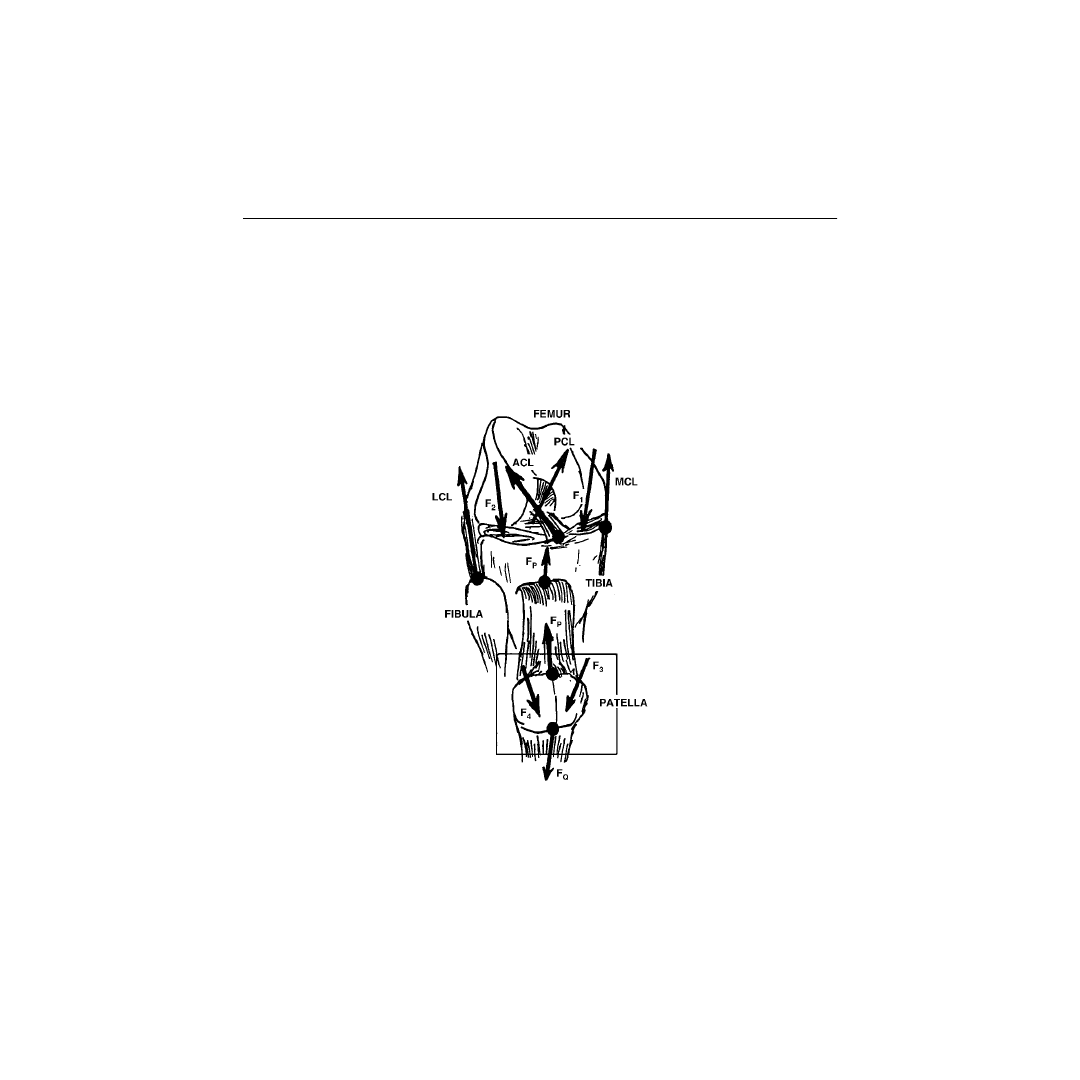
© 2001 by CRC Press LLC
the conditions tested, it could be enough to reconstruct the anterior fibers of the PCL to regain the
stability of a PCL deficient knee. On the other hand, regaining stability of an ACL deficient knee would
require the reconstruction of both the anterior and posterior fibers of the ACL since both fiber bundles
carry significant loads for a large range of knee motion.
1.7 Future Work
The initial results presented in this work encourage us to consider this model as a versatile tool for the
study of the internal forces within the knee joint. Future work includes incorporating the patella into
the model and using it to determine knee response under different loading conditions and to predict the
behavior of the joint following ligamentous injuries and different reconstruction procedures. The intro-
duction of the patella into the present model can be achieved by modeling the knee using three rigid
body segments that comprise the tibio-femoral and patello-femoral joints. Some of the forces acting on
the tibia and patella are shown in
. These two bones are connected by an extensible link that
represents the patellar tendon. Similar to the present tibio-femoral model, the femur will be assumed
fixed, and the friction forces between the femur and patella will be neglected.
In the kinematic analysis, a third coordinate system will be identified on the moving patella. The
patello-femoral joint coordinate system
67
will be used to describe patello-femoral motions in terms of
six kinematic parameters: three rotations (patellar flexion-extension, patellar medial-lateral tilt, and
patellar rotation) and three translations (medial-lateral patellar shift, anterior-posterior patellar transla-
tion, and proximal-distal patellar translation).
When writing the equations of motion, two subsystems will be identified: tibio-femoral and patello-
femoral systems. The force in the patellar tendon, F
P
, will be assumed to act as a coupling force between
these two systems. The tendon will be considered a rigid ligament whose length remains constant during
FIGURE 1.26
A general three-dimensional knee model that includes tibio-femoral and patello-femoral joints. The
force in the patellar tendon, F
P
, acts as a coupling force between the system of equations describing tibio-femoral
motions and the system of equations describing patello-femoral motions.

© 2001 by CRC Press LLC
motion. This rigid patellar ligament condition is expressed mathematically as one equation. The force
in this ligament is the coupling force between the two subsystems of equations describing the tibio-
femoral and patello-femoral joint motions. This force,
, is expressed as:
(1.63)
where F
p
is the magnitude of the patellar ligament force and
is the position vector of the tibial
tuberosity in the femoral coordinate system expressed in terms of its local tibial coordinates and the six
unknown kinematic parameters describing the tibio-femoral motions. Similarly,
is the position vector
of the patellar apex in the femoral coordinate system expressed in terms of its local patellar coordinates
and the six unknown kinematic parameters describing the patello-femoral motions.
The patello-femoral contact will be modeled by assuming that a two-point frictionless contact exists
at all times on the medial and lateral sides such that four forces act on the patella at any instant: the force
exerted by the quadriceps muscle, the force in the patellar ligament, and the medial and lateral contact
forces acting on the medial and lateral patellar facets. The patella will be assumed massless; accordingly,
patellar equations of motion reduce to six equilibrium equations.
An analysis similar to that of the tibio-femoral contact will be employed. The position vectors of each
of the two contact points in the femoral and patellar coordinate systems will be related using the rotation
matrix defined in terms of the six unknown kinematic parameters that describe patello-femoral motions.
Writing this relation at each of the two contact points generates six scalar equations which represent the
patello-femoral contact conditions. Furthermore, Eq. (1.3) is also used to enforce the rigid bodies
condition which is expressed mathematically as four equations that represent the geometric compatibility
conditions for the patello-femoral joint.
The system of equations describing patello-femoral motions will thus consist of 17 equations: six
equilibrium equations, six patello-femoral contact conditions, four patello-femoral compatibility condi-
tions and one rigid patellar ligament condition. Combining both systems we obtain, for the two-point
tibio-femoral contact situation, a system of 33 differential algebraic equations in the following 33
unknowns: (1) six motion parameters describing tibio-femoral joint motions; (2) six motion parameters
describing patello-femoral joint motions; (3) eight parameters representing the
x
and
y
coordinates of
each of the two tibio-femoral contact points in both femoral and tibial systems; (4) eight parameters
representing the
x
and
y
coordinates of each of the two patello-femoral contact points in both patellar
and femoral systems; (5) two parameters representing the magnitude of the tibio-femoral contact forces;
(6) two parameters representing the ratios of the two patello-femoral contact forces to the quadriceps
tendon force; and (7) one parameter describing the ratio of the patellar tendon force to the quadriceps
tendon force.
As a first step, and in order to simplify the solution algorithm of this general model (which involves
solving 33 nonlinear differential algebraic equations), an iterative and approximate procedure can be
adopted in which the tibio-femoral and patello-femoral systems of equations can be solved concurrently.
The solution consists of finding the position of the patella for a given tibial position. Thus, the nonlinear
differential algebraic equations describing the tibio-femoral system will be solved first. The nonlinear
algebraic equations describing the equilibrium of the patella will then be solved to determine the position
of the patella along with the patellar ligament force which acts as the coupling force between the tibio-
femoral and patello-femoral systems.
In this approximate procedure, the initial conditions require the specification of the six kinematic
parameters describing the tibio-femoral motions, and the eight parameters specifying the local
x
and
y
coordinates of the medial and lateral contact points in both femoral and tibial coordinate systems of
axes. These initial values must satisfy the tibio-femoral contact and compatibility equations. Knowing
the initial tibio-femoral position, the initial position of the tibial tuberosity with respect to the femoral
origin can be calculated and then used in conjunction with the quadriceps muscle force as part of the
r
F
p
F
R
R
R
R
p
a
t
a
t
→
→
→
→
→
=
−
−
F
p
r
R
a
r
R
t

© 2001 by CRC Press LLC
patello-femoral input data to solve the patello-femoral system of equations for the initial position of the
patella. The quadriceps force is an input to this system and must be specified as an external load.
The solution of the patello-femoral system of equations provides the initial position of the patellar
apex with respect to the femoral origin and the initial value of the patellar ligament force. The initial
values of these variables are then used as input to a DAE solver to find the solution of the tibio-femoral
system of equations after a time step
∆
t. Knowing the tibio-femoral motions after the time step
∆
t, the
position of the tibial tuberosity with respect to the femoral origin can be calculated at the end of this
time interval. This new position of the tibial tuberosity is then used as part of a new set of patello-femoral
input data to solve the patello-femoral system of equations after a time step
∆
t at which the value of the
quadriceps tendon force is evaluated from the input function at the new time station. The subsequent
solution of the patello-femoral system of equations provides the position of the patellar apex with respect
to the femoral origin and the value of the patellar ligament force after a time step
∆
t. The values of these
two variables are then used as input to find the solution of the tibio-femoral system of equations after a
second time step
∆
t, that is, at time station 2
∆
t. This iterative process continues until the motion is
tracked over the complete range of motion.
Acknowledgment
Part of this work was supported by grants BCS 9209078 and BES 9809243 from the Biomedical Program
of the Biomedical Engineering and Environmental Systems Division of the National Science Foundation.
A portion of this chapter was prepared while Dr. Hefzy was on leave at the Department of Biological
and Medical Research, King Faisal Specialist Hospital and Research Centre, Riyadh, Kingdom of Saudi
Arabia.
References
1. Abdel-Rahman, E., A two-dimensional dynamic model of the human knee joint, Master’s thesis,
University of Toledo, Toledo, OH, 1991.
2. Abdel-Rahman, E. and Hefzy, M.S., Two-dimensional dynamic model of the tibio-femoral joint,
Adv. Bioeng.,
20, 413, 1991.
3. Abdel-Rahman, E. and Hefzy, M.S., A two-dimensional dynamic anatomical model of the human
knee joint,
ASME J. Biomechanical Eng.,
115, 357, 1993.
4. Abdel-Rahman, E. and Hefzy, M.S., Three-dimensional dynamic modeling of the tibio-femoral
joint,
Adv. Bioeng.,
26. 315, 1993.
5. Abdel-Rayman, E., Afjeh, A., and Hefzy, M.S., An improved solution algorithm for the determi-
nation of the 3-D dynamic response of the tibio-femoral joint, Proceedings of the 13th Southern
Biomedical Engineering Conference, April 1994, 368.
6. Abdel-Rahman, E., Hefzy, M.S., and Afjeh, A., Determination of the three-dimensional dynamic
response of the tibio-femoral joint using a DAE solver,
Adv. Bioeng.
, 28, 421, 1994.
7. Abdel-Rahman, E., A three-dimensional dynamic anatomically based model of the human tibio-
femoral joint, Doctoral dissertation, University of Toledo, Toledo, OH, 1995.
8. An, K.-N., Berglund, L., Cooney, W.P., Chao, E.Y.S., and Kovacevic, N., Direct
in vivo
tendon force
measurement system,
J. Biomechanics
, 23, 1269, 1990.
9. Andriacchi, T.P., Mikosz, R.P., Hampton, S.J., and Galante, J.O., Model studies of the stiffness
characteristics of the human knee joint,
J. Biomechanics
, 16, 23, 1983.
10. Arms, S., Boyle, J., Johnson, R., and Pope, M., Strain measurement in the medical collateral
ligament of the human knee: an autopsy study,
J. Biomechanics
, 16, 491, 1983.
11. Arms, S.W., Pope, M.H., Johnson, R.J., Fisher, R.A., Arvidsson, I., and Eriksson, E., The biome-
chanics of anterior cruciate ligament rehabilitation and reconstruction,
Am. J. Sports Med
., 12, 8,
1984.

© 2001 by CRC Press LLC
12. Ateshian, G.A., Soslowsky, L.J., and Mow, V.C., Quantitation of articular surface topography and
cartilage thickness in knee joints using stereophotogrammetry,
J. Biomechanics
, 24, 776, 1991.
13. Ateshian, G.A., A B-spline least-squares surface-fitting method for articular surfaces of diarthrodial
joints,
ASME J. Biomechanical Eng
., 115, 366, 1993.
14. Ateshian, G.A., Kwak, S.D., Soslowsky, L.J., and Mow, V.C., A stereophotogrammetric method for
determining
in situ
contact areas in diarthrodial joints and a comparison with other methods,
J.
Biomechanics
, 27, 111, 1994.
15. Bathe, K.J.,
Finite Element Procedures in Engineering Analysis
, Prentice-Hall, Englewood Cliffs, 1982.
16. Bathe, K.J. and Cimento, A.P., Some practical procedures for the solution of nonlinear finite element
equations,
Computational Methods Appl. Mech. Eng
., 22, 59, 1980.
17. Bendjaballah, M.Z., Shirazi-Adl, A., and Zukor, D.J., Biomechanics of the human knee joint in
compression: reconstruction, mesh generation and finite element analysis,
Knee,
2, 69, 1995
.
18. Beynnon, B.D., Pope, M.H., Fleming, B.C., Howe, J.G., Johnson, R.J., Erickson, A.R., Wertheimer,
C.M., and Nichols, C., An
in vivo
study of the ACL strain biomechanics in normal knee,
Trans.
Orthopaed. Res. Soc
., 14, 324, 1989.
19. Blankevoort, L., Huiskes, R., and deLange, A., The envelope of passive knee joint motion,
J.
Biomechanics
, 21, 705, 1988.
20. Blankevoort, L., Huiskes, R., and deLange, A., Recruitment of knee joint ligaments,
ASME J.
Biomechanical Eng.,
113, 94, 1991.
21. Blankevoort, L. and Huiskes, R., Ligament-bond interaction in a three-dimensional model of the
knee,
ASME J. Biomechanical Eng.,
113, 263, 1991.
22. Blankevoort, L. and Huiskes, R., Parametric validation of a 3-D knee joint model,
J. Biomechanics
,
24, 488, 1991.
23. Blankevoort, L., Kuiper, J.H., Huiskes, R., and Grootenboer, H.J., Articular contact in a three-
dimensional model of the knee,
J. Biomechanics
, 24, 1019, 1991.
24. Brenan, K.E., Campbell, S.L., and Petzold, L.R.,
Numerical Solution of Initial Value Problems in
Differential-Algebraic Equations
, North Holland/Elsevier, Amsterdam, 1989.
25. Biczek, F.L. and Cavanaugh, P.R., Stance phase knee and ankle kinematics and kinetics during level
and down-hill running,
Med. Sci. Sports Exercise
, 22, 669, 1990.
26. Butler, D.L., Groos, E.S., Noyes, F.R., Zernicke, R.F., and Brackett, K., Effects of structure and strain
measurement technique on the material properties of young human tendons and fascia,
J. Biome-
chanics
, 17, 579, 1984.
27. Butler, D.L., Kay, M.D., and Stouffer, D.C., Comparison of material properties in fascicle-bone
units from human patellar tendon and knee ligaments,
J. Biomechanics
, 19, 425, 1986.
28. Butler, D.L., Sheh, M.Y., Stouffer, D.C., Samaranayake, V.A., and Levy, M.S., Surface strain variation
in human patellar tendon and knee cruciate ligaments,
ASME J. Biomechanical Eng.,
112, 39, 1990.
29. Butler, D.L., Guan, Y., Kay, M.D., Cummings, J.F., Feder, S.M., and Levy, M.S., Location-dependent
variations in the material properties of the anterior cruciate ligament,
J. Biomechanics
, 25, 511, 1992.
30. Carlin, G.J., Morrow, D., Harner, C.D., Kusayama, T., and Woo, S.L.-Y., Mechanical properties of
the human posterior cruciate ligament, Proceedings of the 13th Southern Biomedical Engineering
Conference, April 1994, 887.
31. Chand, R., Haug, E., and Rim, K., Stresses in the human knee joint,
J. Biomechanics
, 9, 417, 1976.
32. Chandler, R.F., Clauser, C.E., McConville, J.T., Reynolds, H.M., and Young, J.W., Investigation of
intertial properties of the human body, Report AMRL-TR-74-137, Aerospace Medical Research
Laboratory, Wright-Patterson Air Force Base, OH, March 1975.
33. Cheng, C.K., A mathematical model for predicting bony contact forces and muscle forces at the
knee during human gait, Ph.D. dissertation, University of Iowa, Iowa City, IA, 1988.
34. Clauser, C.E., McConville, J.T., and Young, J.W., Weight, volume, and center of mass of segments
of the human body, Report AMRL-TR-69-70, Aerospace Medical Research Laboratory, Wright-
Patterson Air Force Base, OH, August 1969.

© 2001 by CRC Press LLC
35. Cross, M.J. and Powell, J.F., Long-term follow-up of posterior cruciate ligament rupture: a study
of 116 cases,
Am. J. Sports Med
., 12, 292, 1984.
36. Crowninshield, R., Pope, M.H., and Johnson, R.J., An analytical model of the knee,
J. Biomechanics
,
9, 397, 1976.
37. Crowninshield, R., Pope, M.H., Johnson, R., and Miller, R., The impedance of the human knee,
J. Biomechanics
, 9, 529, 1976.
38. Davy, D.T. and Audu, M.L., A dynamic optimization technique for predicting muscle forces in the
swing phase of the gait,
J. Biomechanics
, 20, 187, 1987.
39. DeLooze, M.P., Toussaint, H.M., van Dieen, H., and Kemper, H.C.G., Joint moments and muscle
activity in the lower extremities and lower back in lifting and lowering tasks, J. Biomechanics, 26,
1067, 1993.
40. Dempster, W.T., Space requirements of the seated operator, Report AD-087-892, Wright-Patterson
Air Force Base, OH, July 1955.
41. van Dijk, R., Huiskes, R., and Selvik, G., Roentgen stereophotogrammetric methods for the eval-
uation of the three-dimensional kinematic behavior and cruciate ligament length patterns of the
human knee joint, J. Biomechanics, 12, 727, 1979.
42. Dortmans, L., Jans, H., Sauren, A., and Huson, A., Nonlinear dynamic behavior of the human
knee joint I. Postmortem frequency domain analyses, ASME J. Biomechanical Eng., 113, 387, 1991.
43. Dortmans, L., Jans, H., Sauren, A., and Huson, A., Nonlinear dynamic behavior of the human
knee joint II. Time-domain analyses: effects of structural damage in postmortem experiments,
ASME J. Biomechanical Eng., 113, 392, 1991.
44. Dufek, J.S. and Bates, B.T., The evaluation and prediction of the impact forces during landings,
Med. Sci. Sports Exercise, 22, 370, 1990.
45. Edwards, R.G., Lafferty, J.F., and Lange, K.O., Ligament strain in the human knee joint, J. Basic
Eng., 92, 131, 1970.
46. Engin, A.E. and Akkas, N., Application of a fluid-filled spherical sandwich shell as a biodynamic
head injury model for primates, Aviation Space Environ. Med., 49, 120, 1978.
47. Engin, A.E. and Moeinzadeh, M.H., Dynamic modelling of human articulating joints, Math.
Modelling, 4, 117, 1983.
48. Engin, A.E. and Tumer, S.T., An innovative approach to the solution of highly nonlinear dynamics
problems associated with joint biomechanics, Proceedings of the 1991 Biomechanics Symposium,
Ohio State University, Columbus, OH, June 1991, 225.
49. Engin, A.E. and Tumer, S.T., Improved dynamic model of the human knee joint and its response
to impact loading on the lower leg, ASME J. Biomechanical Eng., 115, 137, 1993.
50. Essinger, J.R., Leyvraz, P.F., Heegard, J.H., and Robertson, D.D., A mathematical model for the
evaluation of the behavior during flexion of condylar-type knee prostheses, J. Biomechanics, 22,
1229, 1989.
51. Figgie, H.E., Bahniuk, E.H., Heiple, K.G., and Davy, D.T., The effects of tibial-femoral angle on
the failure mechanics of the canine anterior cruciate ligament, J. Biomechanics, 19, 89, 1986.
52. France, E.P., Daniels, A.U., Globe, E.M., and Dunn, H.K., Simultaneous quantitation of knee
ligament forces, J. Biomechanics, 16, 553, 1983.
53. Gear, C.W. and Petzold, L.R., ODE methods for the solution of differential/algebraic systems, SIAM
J. Numer. Anal., 21, 716, 1984.
54. Gear, C.W., Leimkuhler, B., and Gupta, G.K., Automatic integration of Euler-Lagrange equations
with constraints, J. Comp. Appl. Math., 12, 77, 1985.
55. Gear, C.W. and Petzold, L.R., Differential-algebraic equation index transformations, SIAM J. Sci.
Stat. Comp., 9, 39, 1988.
56. Gerald, C.F. and Wheatley, P.O., Applied Numerical Analysis, Addison-Wesley, Reading, 1989, 132.
57. Gill, H.S. and O’Connor, J.J., Biarticulating two-dimensional computer model of the human
patello-femoral joint, Clin. Biomechanics, 11, 81, 1996.

© 2001 by CRC Press LLC
58. Girgis, F.G., Marshall, J.L., and Al Monajem, A.R.S., The cruciate ligaments of the knee joint, Clin.
Orthop., 106, 216, 1975.
59. Glos, D.L., Butler, D.L., Groos, E.S., and Levy, M.S., In vitro evaluation of an implantable force
transducer (IFT) in a patellar tendon model, ASME J. Biomechanical Eng., 115, 335, 1993.
60. Grood, E.S. and Hefzy, M.S., An analytical technique for modeling knee joint stiffness I. Ligamen-
tous forces, ASME J. Biomechanical Eng., 104, 330, 1982.
61. Grood, E.S. and Suntay, W.J., A joint coordinate system for the clinical description of three-
dimensional motions: application to the knee, ASME J. Biomechanical Eng., 105, 136, 1983.
62. Grood, E.S., Hefzy, M.S., and Lindenfield, T.N., Factors affecting the region of most isometric
femoral attachments I. The posterior cruciate ligament, Am. J. Sports Med., 17, 197, 1989.
63. Hatze, H., The meaning of the term biomechanics, J. Biomechanics, 7, 189, 1974.
64. Heegaard, J., Leyvraz, P.F., Curnier, A., Rakotomana, L., and Huiskes, R., Biomechanics of the
human patella during passive knee flexion, J. Biomechanics, 28, 1265, 1995.
65. Hefzy, M.S. and Grood, E.S., Sensitivity of insertion locations on length patterns of anterior cruciate
ligament fibers, ASME J. Biomechanical Eng., 108, 73, 1986.
66. Hefzy, M.S. and Grood, E.S., Review of knee models, Appl. Mechanics Rev., 41, 1, 1988.
67. Hefzy, M.S., Jackson, W.T., Saddemi, S.R., and Hsieh, Y.F., Effects of tibial rotations on patellar
tracking and patello-femoral contact area, J. Biomed. Eng., 14, 329, 1992.
68. Hefzy, M.S. and Yang, H., A three-dimensional anatomical model of the human patello-femoral
joint to determine patello-femoral motions and contact characteristics, J. Biomed. Eng., 15, 289,
1993.
69. Hafzy, M.D. and Abdel-Rahman, E., Dynamic modeling of the human knee joint: formuation and
solution techniques, Biomed. Eng. Appl. Basis Commun., 7, 5, 1995.
70. Hefzy, M.S. and Cooke, T.D.V., A review of knee models: 1996 update, Appl. Mech. Rev., 49, S187,
1996.
71. Hindmarsh, A.C., ODEPACK, a systematized collection of ODE solvers, in Scientific Computing,
Vol. 1, Stepleman, R.S. et al., Eds., North-Holland, Amsterdam, 1983, 55.
72. Hirokawa, S., Three-dimensional mathematical model analysis of the patello-femoral joint, J.
Biomechanics, 24, 659, 1991.
73. Hof, A.L., Pronk, C.N.A., and van Best, J.A., Comparison between EMG to force processing and
kinetical analysis for the calf muscle moment in walking and stepping, J. Biomechanics, 20, 167,
1987.
74. Hughston, J.C., Bowden, J.A., Andrews, J.R., and Norwood, L.A., Acute tears of the posterior
cruciate ligament, J. Bone Joint Surg., 62-A, 438, 1980.
75. Huiskes, R. and Blankevoort, L., The relationship between knee joint motion and articular surface
geometry, in Biomechanics of Diarthrodial Joints, Vol. 2, Springer-Verlag, New York, 1990, 269.
76. Huson, A., Biomechanische Probleme des Kniegelenks, Orthopaede, 3, 119, 1974.
77. Jackson, K.R. and Sacks-Davis, R., An alternative implementation of variable step-size multistep
formulae for stiff ODEs, ACM Trans. Math. Software, 6, 295, 1980.
78. Jans, H.W.J., Dortmans, L.J.M.G., Sauren, A.A.H.J., and Huson, A., An experimental approach to
evaluate the dynamic behavior of the human knee, ASME J. Biomechanical Eng., 110, 69, 1988.
79. van Kampen, A., The three-dimesional tracking pattern of the patella, Ph.D. dissertation, University
of Nijmegen, The Netherlands, 1987.
80. Kao, R., A comparison of Newton-Raphson methods and incremental procedures for geometrically
nonlinear analysis, Comp. Struc., 4, 1091, 1974.
81. Kaufman, K.R., Muscle and joint forces in the knee during isokinetic exercise, J. Biomechanics, 23,
711, 1990.
82. LaFortune, M.A., Cavanagh, P.R., Summer, H.J., and Kalenak, A., Three-dimensional kinematics
of the knee during walking, J. Biomechanics, 25, 347, 1992.
83. Lindbeck, L., Impulse and moment of impulse in the leg joints by impact from kicking, ASME J.
Biomechanical Eng., 105, 108, 1983.

© 2001 by CRC Press LLC
84. Ling, Z.-K., Guo, H.-Q., and Boersma, S., Analytical study on the kinematic and dynamic behaviors
of a knee joint, Med. Eng. Phys., 19, 29, 1997.
85. Loos, W.C., Fox, J.M., Blazina, M.E., Del Pizzo, W., and Friedman, M.J., Acute posterior cruciate
ligament injuries, Am. J. Sports Med., 9, 86, 1981.
86. MacKinnon, C.D. and Winter, D.A., Control of the whole body balance in the frontal plane during
human walking, J. Biomechanics, 26, 633, 1993.
87. Macquet, P.G., Van De Berg, A.J., and Simonet, J.C., Femorotibial weight-bearing areas: experi-
mental determination, JBJS, 57-A, 766, 1975.
88. Menschik, A., Mechanik des Kniegelenkes, Teil 1, Z. Orthoped., 112, 481, 1974.
89. Menschik, A., Mechanik des Kniegelenkes, Teil 2, Z. Orthoped., 113, 388, 1975.
90. Menschik, A., The basic kinematic principle of the collateral ligaments, demonstrated on the knee
joint, in Injuries of the Ligaments and Their Repair, Chapchal, G., Ed., Thieme, Stuttgart, 1977, 9.
91. Mills, O.S. and Hull, M.L., Apparatus to obtain rotational flexibility of the human knee under
moment loads in vivo, J. Biomechanics, 24, 351, 1991.
92. Mills, O.S. and Hull, M.L., Rotational flexibility of the human knee due to various varus/valgus
and axial moments in vivo, J. Biomechanics, 24, 673, 1991.
93. Moeinzadeh, M.H., Two- and three-dimensional dynamic modeling of the human joint structures
with special application to the knee joint, Ph.D. dissertation, Ohio State University, Columbus,
OH, 1981.
94. Moeinzadeh, M.H., Engin, A.E., and Akkas, N., Two-dimensional dynamic modeling of the human
knee joint, J. Biomechanics, 16, 253, 1983.
95. Moeinzadeh, M.H. and Engin, A.E., Response of a two-dimensional dynamic model to externally
applied forces and moments, J. Biomedical Eng., 105, 281, 1983.
96. Moeinzadeh, M.H. and Engin, A.E., Dynamic modeling of the human knee joint, in Computational
Methods in Bioengineering, Vol. 9, American Society of Mechanical Engineering, Chicago, 1988, 145.
97. Moffat, C.A., Harris, E.H., and Haslam, E.T., An experimental and analytical study of the dynamic
properties of the human leg, J. Biomechanics, 2, 373, 1969.
98. Morrison, J.B., The mechanics of the knee joint in relation to normal walking, J. Biomechanics, 3,
51, 1970.
99. Mow, V.C., Ateshian, G.A., and Spilker, R.L., Biomechanics of diarthrodial joints: a review of twenty
years of progress, ASME J. Biomechanical Eng., 115, 460, 1993.
100. Muller, W., The Knee: Form, Function and Ligament Reconstruction, Springer-Verlag, Berlin, 1982.
101. Muller, W., Kinematics of the cruciate ligaments, in The Cruciate Ligaments, Feagin, J.A., Jr., Ed.,
Churchill Livingstone, New York, 1988.
102. Mungiole, M. and Martin, P.E., Estimating segment inertial properties: comparison of magnetic
resonance imaging with existing methods, J. Biomechanics, 23, 1039, 1990.
103. Nigg, B.M., Cole, G.K., and Nachbauer, W., Effects of arch height of the foot on angular motion
of the lower extremities in running, J. Biomechanics, 26, 909, 1993.
104. Ogata, K., McCarthy, J.A., Dunlap, J., and Manske, P.R., Pathomechanics of posterior sag of the
tibia in posterior cruciate deficient knees: an experimental study, Am. J. Sports Med., 16, 630, 1988.
105. Petzold, L.R., Differential/algebraic equations are not ODEs, SIAM J. Sci. Stat. Comput., 3, 367,
1982.
106. Petzold, L.R., A description of DASSL: a differential/algebraic system solver, in Scientific Computing,
Vol. 1, Stepleman, R.S. et al., Eds., North-Holland, Amsterdam, 1983, 65.
107. Platt, D., Wilson, A.M., Timbs, A., Wright, I.M., and Goodship, A.E., Novel force transducer for
the measurement of tendon force in vivo, J. Biomechanics, 27, 1489, 1994.
108. Pope, M.H., Crowninshield, R., Miller, R., and Johnson, R., The static and dynamic behavior of
the human knee in vivo, J. Biomechanics, 9, 449, 1976.
109. Race, A. and Amis, A.A., The mechanical properties of the two bundles of the human posterior
cruciate ligament, J. Biomechanics, 27, 13, 1994.

© 2001 by CRC Press LLC
110. Radin, E.L. and Paul, I.L., A consolidated concept of joint lubrication, J. Bone Joint Surg., 54-A,
607, 1972.
110a. Rahman, E.M. and Hefzy, M.S., Three-dimensional dynamic behaviour of the human knee joint
under impact loading, JJBE: Med. Eng. Phys., 20, 4, 1998.
111. Rogers, G.J., Milthorpe, B.K., Muratore, A., and Schindhelm, K., Measurement of mechanical
properties of the anterior cruciate ligament, Aust. J. Phys. Eng., 8, 168, 1985.
112. Rohrle, H., Scholten, R., Sigolotto, C., Solbach, W., and Kellner, H., Joint forces in the human
pelvis-leg skeleton during walking, J. Biomechanics, 17, 409, 1984.
113. Seedhom, B.B., Dowson, D., and Wright, V., The load-bearing function of the menisci: preliminary
study, in The Knee Joint, Proceedings of the International Congress, Excerpta Medica, Rotterdam,
1974, 37.
114. Seireg, A. and Arvikar, R.J., The prediction of muscular load sharing and joint forces in the lower
extremities during walking, J. Biomechanics, 8, 89, 1975.
115. van Soest, A.J., Schwab, A.L., Bobbert, M.F., and van Ingen-Schenau, G.J., The influence of the
biarticularity of the gastrocnemius muscle on vertical jumping achievement, J. Biomechanics, 26,
1, 1993.
116. Soslowsky, L.J., Flatow, E.L., Bigliani, L.U., and Mow, V.C., Articular geometry of the glenohumeral
joint, Clin. Orthopedics Rel. Res., 285, 181, 1992.
117. Takai, S., Woo, S.L.-Y., Livesay, G.A., Adams, D.J., and Fu, F.H., Determination of the in situ loads
on the human anterior cruciate ligament, J. Orthopaed. Res., 11, 686, 1993.
118. Tumer, S.T. and Engin, A.E., Three-body segment dynamic model of the human knee, ASME J.
Biomechanical Eng., 115, 350, 1993.
119. Tumer, S.T., Wang, I., and Akkas, N., A planar dynamic anatomic model of the human lower limb,
Biomed. Eng. Appl. Basis Commun., 7, 365, 1995.
120. Vaughan, C.L., Davis, B.L., and O’Connor, J.C., Dynamics of Human Gait, Human Kinetics, Cham-
paign, IL, 1992, 20.
121. Wahrenberg, H., Lindbeck, L., and Ekholm, J., Dynamic load in the human knee joint during
voluntary active impact to the lower leg, Scand. J. Rehabil. Med., 10, 93, 1978.
122. Wahrenberg, H., Lindbeck, L., and Ekholm, J., Knee muscular moment, tendon tension force and
EMG during vigorous movement in man, Scand. J. Rehabil. Med., 10, 99, 1978.
123. Walker, P.S. and Hajek, J.V., The load bearing area in the knee joint, J. Biomechanics, 5, 581, 1972.
124. Walker, P.S., Kurosawa, M.D., Rovick, M.A., and Zimmerman, B.S., External knee joint design
based on normal motion, J. Rehabil. Res. Dev., 22, 9, 1985.
125. Walker, P.S. and Garg, A., Range of motion in total knee arthroplasty: a computer analysis, Clin.
Orthopedics Rel. Res., 262, 227, 1991.
126. Wang, C.J., Walker, P.S., and Wolf, B., The effects of flexion and rotation on the length patterns of
the ligaments of the knee, J. Biomechanics, 6, 587, 1973.
127. Wang, C.J. and Walker, P.S., Rotatory laxity of the human knee joint, J. Bone Joint Surg., 56-A, 161,
1974.
128. Warren, L.F., Marshall, J.L., and Girgis, F., The prime static stabilizer of the medial side of the knee,
J. Bone Joint Surg., 56-A, 665, 1974.
129. Wismans, J., A three-dimensional mathematical model of the human knee joint, Ph.D. dissertation,
Eindhoven University of Technology, Eindhoven, The Netherlands, 1980.
130. Wismans, J., Veldpaus, F., Janssen, J., Huson, A., and Strulen, P., A three-dimensional mathematical
model of the knee joint, J. Biomechanics, 13, 677, 1980.
131. Wongchaisuwat, C., Hemami, H., and Buchner, H.J., Control of sliding and rolling at natural joints,
ASME J. Biomechanical Eng., 106, 368, 1984.
132. Woo, S. L.-Y., Hollis, M., Roux, R.D., Gomez, M.A., Inoue, M., Kleiner, J.B., and Akeson, W.H.,
Effects of knee flexion on the structural properties of the rabbit femur anterior cruciate ligament-
tibia complex (FATC), J. Biomechanics, 20, 557, 1987.

© 2001 by CRC Press LLC
133. Woo, S. L.-Y., Hollis, M., Adams, D.J., Lyon, R.M., and Takai, S., Tensile properties of the human
femur anterior cruciate ligament-tibia complex: the effects of specimen age and orientation, Am.
J. Sports Med., 19, 217, 1991.
134. Woo, S. L.-Y., Johnson, G.A., and Smith, B.A., Mathematical modeling of ligaments and tendons,
ASME J. Biomechanical Eng., 115, 468, 1993.
135. Yasuka, K., Erickson, A.R., Johnson, R.J., and Pope, M.H., Dynamic strain behavior in the medial
collateral and anterior cruciate ligaments during lateral impact loading. Trans. Orthopaed. Res. Soc.,
17, 127, 1992.
136. Zoghi, M., Hefzy, M.S., Jackson, W.T., and Fu, K.C., A three-dimensional morphometrical study
of the distal human femur, J. Eng. Med., 206, 147, 1992.
137. Zoghi, M., Solving the 3-dimensional contact problem between femur and menisci and tibia,
Doctoral dissertation, University of Toledo, Toledo, OH, 1997.
Document Outline
- Musculoskeletal Models and Techniques
- Table of Contents
- Three-Dimensional Dynamic Anatomical Modeling of the Human Knee Joint
Wyszukiwarka
Podobne podstrony:
CH 01 ZMARTWYCHWSTANIE PJ
CH 01 2010 EN
Family in Transition Ch 01
CH 01 ZMARTWYCHWSTANIE PJ
CH 01 2010 EN
GERALD appel ch 01
01 BIOCHEMIA wybrane zagadnienia ch org
Wingrove David Chung Kuo 03 Biała Góra 01 Na Moście Ch in
zasady diagnostyki ch motochondrialnychPiekut Abramczuk 06 01
TD 01
Ubytki,niepr,poch poł(16 01 2008)
9 Ch organiczna WĘGLOWODANY
ch wrzodowa prof T Starzyńska
01 E CELE PODSTAWYid 3061 ppt
01 Podstawy i technika
01 Pomoc i wsparcie rodziny patologicznej polski system pomocy ofiarom przemocy w rodzinieid 2637 p
ch zwyrodnieniowa st
więcej podobnych podstron