Part I: Picking the Right Investment Vehicles

Successful investing involves two basic areas of decision: what do you buy and sell,
and when to buy and sell. We’ll be moving along into the “whens” in chapters to
come, as we develop a broad array of market timing techniques. Before we move
into timing, however, we will consider some principles and procedures that should
prove helpful in selecting vehicles in which to invest.

It’s not how much you make that counts; it’s how much you manage not to lose.
Let’s start by considering just a few numbers. The Nasdaq Composite Index

reached an all-time high on March 6, 2000, closing that day at 5048.60. The ensuing
bear market took the index down to a low of 1,114.40 on October 9, 2002—a loss of
77.9%. Prices advanced from that point. By December 3, 2003, the Composite had
risen to 1960.20that’s 75.9% above the lows of October, 2002. And where did the buy-
and-hold investor stand at that point? Down—very much down still, by 61.2% from
the March 2000 close!

The moral: To make up any losses taken in the stock market, you have to achieve

greater percentage gains than such losses entail. It does not matter whether the losses
or the gains come first.

For example, if you lose 20% of the value of your assets, you have to make 25%

on the remainder to break even. (If you start with $100,000 and lose 20%, you have
$80,000. To bring that $80,000 back to $100,000, you have to show a gain of $20,000
which represents 25% of the $80,000 you have left in your account.)

1

The No-Frills Investment
Strategy

Appel_01T.qxd 1/26/05 8:14 PM Page 1

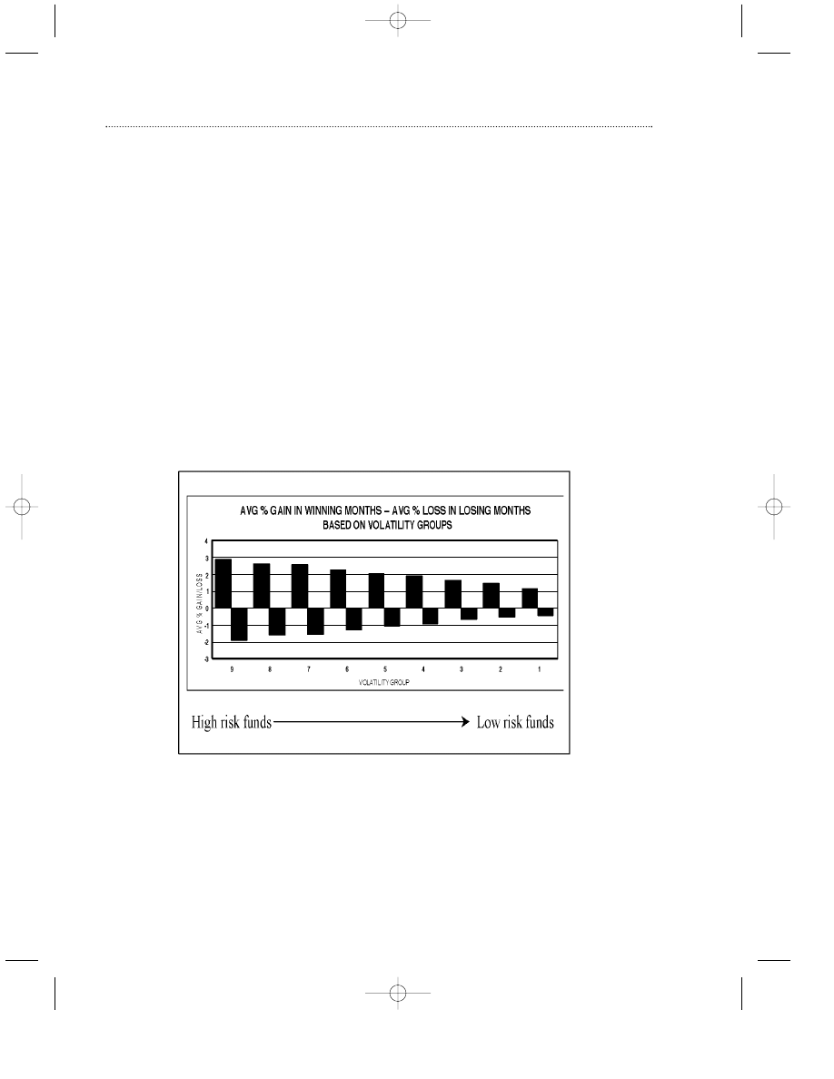
Chart 1.1

Average Percent Gain in Winning Months and Average Percent Loss in Losing

Months, Based on Volatility Groups

This chart shows the average gain during months in which the average mutual fund rose in
price (winning months) compared to months in which the average mutual fund declined (los-
ing months). Mutual funds are ranked by volatility, the amount of daily and/or longer-term

2

Trading Commodities and Financial Futures

If you lose one-third, or 33.33%, of your assets, you will have to make 50% on

your remaining assets to break even. If you make 50% first, a loss of 33.33% will
bring you back to your starting level.

If you lose 25%, you will need to gain 33.33% to bring you back to your starting

level.

If you lose 50%, you will need to make 100% to restore your original capital.
If you lose 77.9%, you will need to make 352.5% on the assets left to break even.
I think you get the idea by now. Capital preservation is, by and large, more

important for successful long-term investment than securing an occasional large
profit. We will, of course, be reviewing a number of timing tools that are designed
to provide more efficient entries and exits into the stock market, thereby reducing
risk and improving the odds of maintaining and growing your capital assets. Let’s
begin, however, with strategies for portfolio selection, which should be very useful
supplements to your market-timing arsenal.

Risk: Reward Comparisons Between More Volatile and Less
Volatile Equity Mutual Fund Portfolios

Appel_01T.qxd 1/26/05 8:14 PM Page 2

The No-Frills Investment Strategy

3

price fluctuation that takes place in that fund, usually compared to the Standard & Poor’s 500
Index as a benchmark. Group 9 represents the most volatile group of funds; Group 1 repre-
sents the least volatile segment. The period represented by this study was December 1983 to
October 2003. The more volatile the group, typically the greater the gain during winning
months, the greater the losses during losing months.

Calculations and conclusions presented in this chapter and in other areas where perform-

ance data is shown are based, unless otherwise mentioned, on research carried forth at
Signalert Corporation, an investment advisory of which the author is sole principal and presi-
dent. In this particular case, research encompassed mutual fund data going back to 1983,
involving, among other processes, simulations of the strategies described for as many as
3,000 different mutual funds, with the number increasing over the years as more mutual funds
have been created.

Chart 1.1 shows the relationships between average percentage gains during rising

months for mutual funds of various volatility levels (range of price fluctuations) and
the average percentage loss during declining market months, 1983 to 2003. For exam-
ple, the most volatile segment of the mutual fund universe employed in this study
(Group 9) gained just less than 3% during months that the average fund in that
group advanced, and incurred an average loss of just less than 2% during months
that the average fund in that group declined. As a comparison, funds in Group 1, the
least volatile segment of this mutual fund universe, advanced by approximately
1.2% on average during rising months for that group and declined by approximate-
ly 4/10 of 1% during months that the average fund in that group showed a decline.

Chart 1.1 shows us that, basically, when more volatile mutual funds—and, by

implication, portfolios of individual stocks that show above-average volatility—are
good, they can be very good, indeed. However, when such portfolios are bad, they
can be very bad, indeed. Are the gains worth the risks? That’s a logical question that
brings us to a second chart.

Gain/Pain Ratios

We have seen that the more aggressive the portfolio, the larger the average gain is
likely to be during rising market periods. We have also seen that more aggressive
portfolios are likely to lose more during declining market periods. That’s logical
enough—nothing for nothing. But what are the gain/pain ratios involved?

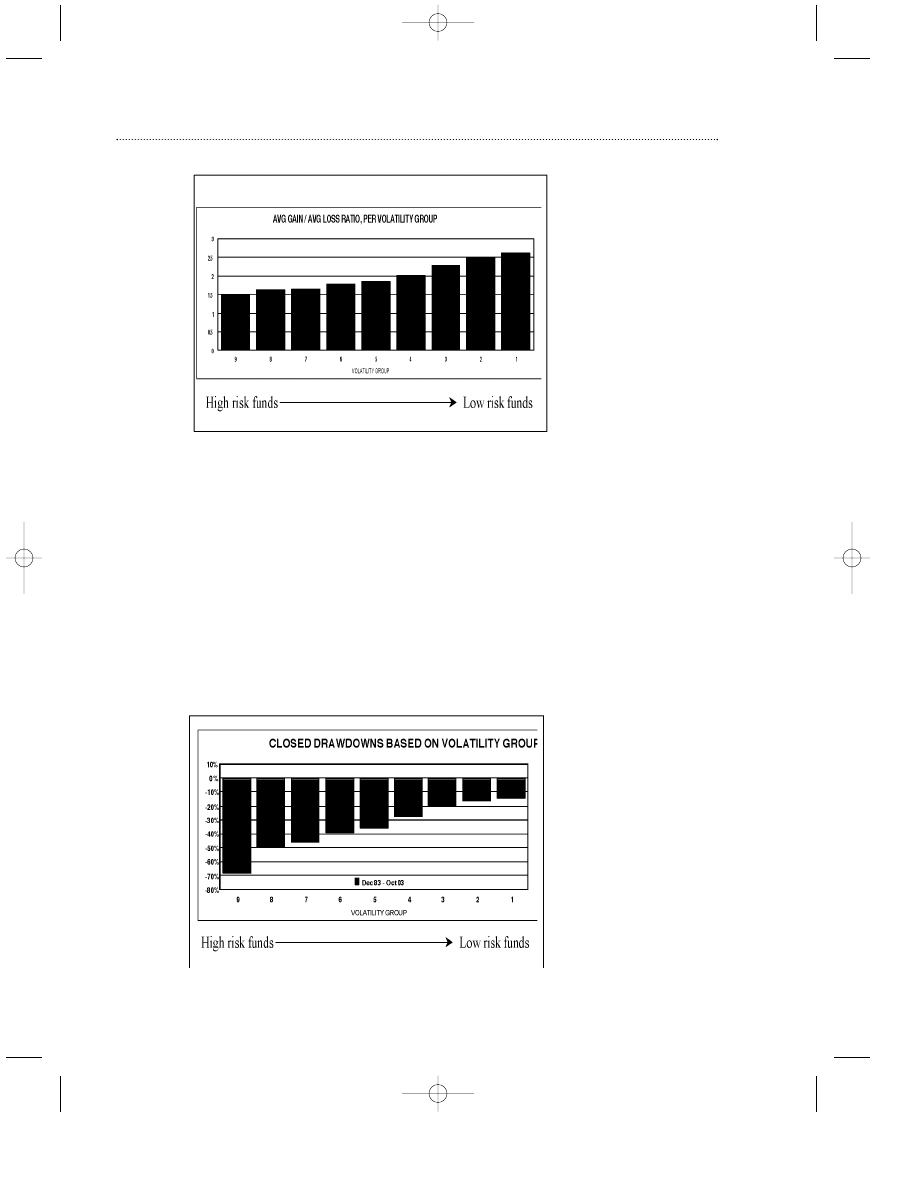
Well, Chart 1.2 shows that, on a relative basis, more volatile mutual funds involve

greater pain to gain, lower profit/loss ratios than less volatile portfolios. For exam-
ple, Group 9, the most volatile portfolio segment, makes about 3% during winning
months for every 2% lost during declining months, a gain/loss ratio of essentially
1.5. Group 1, the least volatile group, has had a gain/loss ratio of approximately 2.7.
You make 2.7% per winning month for every percent of assets lost during losing
months. The amount of extra gain achieved by more volatile funds is offset by the
disproportionate risk assumed in the maintenance of such portfolios.

Appel_01T.qxd 1/26/05 8:14 PM Page 3

4

Trading Commodities and Financial Futures

Chart 1.2

Average Gain/Average Loss, by Volatility Group

This chart shows the ratio of the average gain per winning month to the average loss per los-
ing month, by volatility group. For example, Group 9, the highest-volatility group, shows a
gain/loss ratio of 1.5. Winning months were, on average, 1.5 times the size of losing months.
Group 2, the second-least-volatile group, shows a gain/loss ratio of 2.5. Winning months, on
average, were 2.5 times the size of losing months. The period here was 1983 to 2003.

You might notice that relationships between volatility and risk are very constant

and linear. The greater the volatility, the lesser the gain/loss ratio, the greater the
risk—a relationship frequently lost to investors during periods when speculative
interest in high-volatility stocks runs high.

Drawdown: The Measure of Ultimate Risk

Chart 1.3

Closed Drawdowns by Volatility

Appel_01T.qxd 1/26/05 8:14 PM Page 4

The No-Frills Investment Strategy

5

Drawdown represents the maximum loss taken from a peak in portfolio value to a subsequent
low before a new peak in value is achieved. The highest-volatility group, Group 9, incurred
losses of as much as 68% during the 1983–2003 period, whereas the lowest-volatility group,
Group 1, had a maximum drawdown of just 15%.

Drawdown, the amount by which your portfolio declines from a peak
reading to its lowest value before attaining a new peak, is one of the
truer measures of the risks you are taking in your investment program.

For example, let us suppose that you had become attracted to those highly

volatile mutual funds that often lead the stock market during speculative invest-
ment periods., and therefore accumulated a portfolio of aggressive mutual funds
that advanced between late 1998 and the spring of 2000 by approximately 120%,
bringing an initial investment of $100,000 to $220,000. So far, so good. This portfolio,
however, however, declines by 70% during the 2000–2003 bear market to a value of
$66,000. Although losses of this magnitude to general mutual fund portfolios previ-
ously had not taken place since the 1974 bear market, they have taken place during
certain historical periods and must be considered a reflection of the level of risk
assumed by aggressive investors. Moreover, this potential risk level might have to
be increased if asset values for this portfolio and similar portfolios were to decline to
new lows before achieving new peaks, which had not yet taken place during the first
months of 2004.

Protracted gains in the stock market tend to lead investors to presume that

stock prices will rise forever; buy-and-hold strategies become the strategy of
choice. Interest focuses on gain. Potential pain is overlooked. (Conversely, long
periods of market decline tend to lead investors to minimize the potential of stock
ownership. The emphasis becomes the avoidance of pain; the achievement of gain
seems hopeless.)

Drawdowns—and risk potential—decline dramatically as portfolio volatility

decreases, although risks to capital are still probably higher than most investors real-
ize, even in lower-volatility areas of the marketplace. For example, maximum draw-
downs between 1983 and 2003 were roughly 16% for Group 2, the second-least-
volatile group of mutual funds, rising to 20% in Group 3, a group of relatively low
volatility. Mutual funds of average volatility, Group 5, showed drawdowns of 35%.

In evaluating mutual funds or a selection of individual stocks or ETFs for your

portfolio, you should secure the past history of these components to assess maxi-
mum past risk levels. ETFs (exchange traded funds) are securities, backed by relat-
ed baskets of stocks, which are created to reflect the price movement of certain stock
market indices and/or stock market sectors. For example, there are ETFs called SPY-
DRS that reflect the price movement of the Standard & Poor’s 500 Index, rising and
falling in tandem with the index. Another ETF, the QQQs, reflects the Nasdaq 100
Index. There are ETFs that reflect a portfolio of high-yielding issues in the Dow
Industrial Average, a real estate trust portfolio, and even an ETF that reflects a port-
folio of 10-year Treasury bonds. In many ways, ETFs are similar to index- or sector-
based mutual funds, have the advantages of unlimited trading at any time of the
day, as well as lower internal expenses than mutual funds. There are certain disad-
vantages, however, mainly associated with bid-ask spreads, which add to transac-
tion costs as well as occasional periods of limited liquidity.

Appel_01T.qxd 1/26/05 8:14 PM Page 5

Chart 1.4

Twenty Years of Results, Based on Volatility Group

All things considered, investors gain little, if anything, by placing investments in higher-risk
holdings. Lower-volatility groups have provided essentially the same investment results over
the long run as higher-volatility groups, but with much less risk.

Chart 1.4 pretty much tells the story. With the exception of mutual funds in Group 1
(which includes many hybrid stock, bond funds), equity and balanced mutual funds
of relatively low volatility produced essentially the same returns over the 1983–2003
decade as mutual funds of higher volatility. Generally, the highest average returns
were secured with mutual funds of approximately average volatility, where the
curve of returns appears to peak. However, differentials in return between Groups
2–3 and Groups 4–6 might or might not justify the increases in risk that are involved
in stepping up from the very low-volatility groups to those at the average level.

To sum up, for buy-and-hold strategies, higher volatility has historically pro-

duced little, if any, improvement in return for investors, despite the greater risks
involved. These actual results run counter to the general perception that investors
can secure higher rates of return by accepting higher levels of risk, an assumption
that might be correct for accurate and nimble market traders during certain periods
but, in fact, is not the case for the majority of investors, who are most likely to posi-
tion in aggressive market vehicles at the wrong rather than the right times.

6

Trading Commodities and Financial Futures

You can fine-tune the total risk of your total portfolio by balancing its compo-

nents to include lower-risk as well as higher-risk segments. For example, a mutual
fund portfolio consisting 50% of intermediate bond funds (past maximum draw-
down 10%) and 50% Group 8 mutual funds (past maximum drawdown 50%), would
represent a total portfolio with a risk level of approximately 30%, probably as much,
if not more, risk than the typical investor should assume.

The End Result: Less Is More:

Appel_01T.qxd 1/26/05 8:14 PM Page 6

The No-Frills Investment Strategy

7

Lower-volatility mutual funds typically produce higher rates of return and less

drawdown, something to think about.

Inasmuch as accurate timing can reduce the risks of trading in higher-velocity

equities, active investors can employ more volatile investment vehicles if they man-
age portfolios in a disciplined manner with efficient timing tools. Relative returns
compared to lower-volatility vehicles improve. Aggressive investors with strong
market-timing skills and discipline might find it worthwhile to include a certain
proportion of high-velocity investment vehicles in their portfolios—a certain pro-
portion, perhaps up to 25%, but not a majority proportion for most.

Again, we will continue to consider tools that will improve your market timing.

However, before we move into that area, I will show you one of the very best strate-
gies I know to maintain investment portfolios that are likely to outperform the aver-
age stock, mutual fund, or market index.

Changing Your Bets While the Race Is Still Underway

Let’s suppose you have a choice.

You go to the racetrack to bet on the fourth race, research the history of the hors-

es, evaluate the racing conditions, check out the jockeys, evaluate the odds, and
finally buy your tickets. Your selection starts well enough but, by the first turn, starts
to fade, falling back into the pack, never to re-emerge; your betting capital disap-
pears with the horse. The rules of the track, of course, do allow you to bet on more
than one horse. The more horses you bet on, the greater your chances are that one
will come through or at least place or show, but then there are all those losers....

Then you find a track that offers another way to play. You may start by betting

on any horse you choose, but at the first turn, you are allowed to transfer the initial
bet—even transfer your bet to the horse leading at the time. If the horse is still lead-
ing at the second turn, you will probably want to hold your bet. If the horse falters,
however, you are allowed to shift your bet again, even to the horse that has just
taken the lead. Same at the third turn. Same at the final turn. You can stay with the
leaders, if you like, or, if your horse falls back into the pack, you can move the bet
to the new leading horse until the race comes to an end. (I have, of course, taken
some liberties with the analogies, to make a point.)

Which way do you think you’d prefer? Betting and holding through thick and

thin, and, perhaps, through your horse running out of steam? Or shifting bets at
each turn so your money starts each turn riding on a leading horse?

The first track is a little like the stock market, whose managers seem always to be

telling investors what to buy, sometimes when to buy, but rarely, if ever, when to
change horses. Buy-and-hold strategies do have their benefits, particularly over the
very long term. It is possible, after all, for all stock market investors to make money
in the end, which is not true for all bettors at the track.

The second track, however, is more likely to give an edge to the player. Strong

horses tend to remain strong, especially when you don’t have to ride them to the fin-
ish line if they begin to lose serious ground. That brings us to relative strength
investing.

Appel_01T.qxd 1/26/05 8:14 PM Page 7

8

Trading Commodities and Financial Futures

Relative Strength Investing

The basic principles of relative strength investing:

• Identify the leaders.

• Buy the leaders.

• Hold the leaders for as long as they lead.

• When the leaders slow down, sell them and buy new leaders.

Simple enough?
Let’s get more specific.

For investors of average to below average risk tolerance, start by securing a data-

base or two of a large number of mutual funds. I prefer a database of at least 1,000
mutual funds—preferably more, but for the purposes of a single investor instead of
a capital manager, a few hundred is almost certainly sufficient.

You need quarterly data, so almost any source that tracks mutual funds and pro-

vides quarterly performance data serves your purpose. Barron’s, the Dow Jones
Business and Financial Weekly, for example, provides good coverage. Other sources
can be found on the Web.

For example, in the Finance areas of Yahoo.com and MSN.com, you can find

charts and information regarding mutual funds. A number of investment advisory
newsletters provide performance and other information regarding mutual funds.
Newsletters that provide recommendations and data specific to the sort of invest-
ment approach I am suggesting include my own newsletter, Systems and Forecasts,
and the newsletter No-Load Fund X. You can find information regarding these pub-
lications www.Signalert.com and www.NoloadfundX.com, respectively.

Conservative investors should eliminate from the array of funds covered those

that are normally more volatile than the Standard & Poor’s 500 Index. Such funds
often provide excellent returns during strong and speculative market climates, but
you will probably secure better balances between risk and reward if you concentrate
your selections on mutual funds that are, at most, just somewhat above (preferably
approximately equal to or below) the Standard & Poor’s 500 Index in volatility. Your
portfolio, when fully invested, will probably include holdings that are, on average,
approximately 80–85% as volatile (risky) as the Standard & Poor’s 500 Index. Actual
risk is likely to be reduced below these ratios as a result of the exceptional relative
strength of your holdings. (More on this comes shortly.)

When you have isolated a universe of mutual funds whose volatility is more or

less equal to or less than the Standard & Poor’s 500 Index—for example, the Dodge
and Cox Balanced Fund and First Eagle Sogen—determine from the performance
tables which funds have shown performance results over the past three months
that rank in the upper 10% (top decile) of all the mutual funds of similar volatility
in your database. These are funds that have shown the greatest percentage gain for
the period.

Buy a selection of at least two—preferably four or five—funds in the top decile of

the mutual fund universe that consists of funds of equal or less volatility than the
Standard & Poor’s 500 Index. Some level of diversification is significant. Even a

Appel_01T.qxd 1/26/05 8:14 PM Page 8

portfolio of as little as two mutual funds provides considerable increase in safety
compared to a single-fund portfolio. Look for funds that charge no loads for pur-
chase and involve no redemption fees for holding periods of at least 90 days.

Review your portfolios every three months, as new quarterly data becomes avail-

able. If any funds have fallen from the top decile, sell those funds and replace them
with funds that remain or have just entered into the top decile in performance.
Maintain current holdings that retain their positions in the top 10% of performance
of all mutual funds of that volatility group.

Funds should be ranked against their own volatility peers. During rising market

periods, funds of higher volatility tend to outperform funds of lower volatility sim-
ply because higher-volatility mutual funds and stocks tend to move more quickly
than funds and stocks of lower volatility. Conversely, higher-volatility positions
tend, on average, to decline more quickly in price than lower-volatility vehicles. We
are seeking funds that produce the best returns for varied market climates, includ-
ing both advancing and declining market periods. You can secure volatility ratings
of mutual funds from a variety of sources, including Steele Mutual Fund Expert (see
www.mutualfundexpert.com), an excellent reference for mutual fund information.

If you follow this procedure, you will regularly rebalance and reapportion your

mutual fund holdings so that, at the start of every quarter, you will hold a portfolio
of mutual funds that have been leading their peer universe in strength. Your portfo-
lio will consist of mutual funds with the highest relative performance, horses that
are leading the pack at every turn of the course.

Testing the Relative Strength Investment Strategy: A Fourteen-Year
Performance Record of Relative Strength Investing

The No-Frills Investment Strategy

9

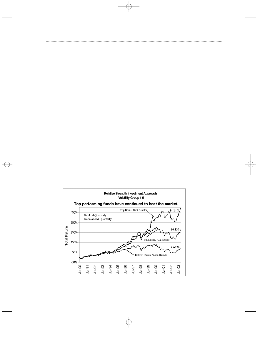
Chart 1.5

Performance of the Relative Strength Investment Approach (1990–2003)

Appel_01T.qxd 1/26/05 8:14 PM Page 9

10

Trading Commodities and Financial Futures

This chart shows the performance of ten performance deciles of mutual funds from 1990 to
2003. The assumption is made that, at the start of each quarter, assets are rebalanced so that
investments are made only in funds that are ranked in the top 10% of performance for the
previous quarter among mutual funds whose volatilities were equal to or less than the volatili-
ty of the Standard & Poor’s 500 Index. The initial universe in 1990 was approximately 500
funds, increasing over the years to more than 3,000 by 2003. Performance was very consis-
tent with rankings. This chart is based upon hypothetical research.

Chart 1.5 shows the results of a hypothetical back-test of this procedure of main-
taining a portfolio of mutual funds of average to below-average volatility, reranking
in performance each quarter, reallocating your holdings at that time by selling posi-
tions that have fallen from the top 10% in performance, and selecting and replacing
such positions from those funds that have remained or recently entered into the
upper decile.

Again, it goes without saying that this program should be carried out with no-

load mutual funds that charge redemption fees only if assets are held less than 90
days. Brokerage firms such as Schwab and T. D. Waterhouse, as well as many oth-
ers, provide platforms of no-load mutual funds from which you can make selec-
tions. Our research universe included equity, balanced, and sector mutual funds.
Your own universe can be similarly created.

Rebalancing can take place more frequently than at 90-day intervals, if you pre-

fer. For example, somewhat higher rates of return appear to accrue when ranking
and rebalancing procedures take place at monthly rather than quarterly intervals.
However, more frequent portfolio rotations result in increased trading expenses and
probable increases in mutual fund redemption fees, all of which could well offset the
advantages gained by more frequent portfolio reallocation. A program of rebalanc-
ing at intervals of more than three months is also likely to provide considerable ben-
efit, although returns are likely to diminish somewhat as a result.

There is another significant reason to reduce trading frequency. As a result of

scandals during 2003 and 2004 that took place related to mutual fund timing, mutu-
al fund management companies and the distribution network of mutual funds
became more sensitive to frequent trading by active market timers as a source of
possible fund disruption. Close monitoring of active investors has become the norm,
with frequent traders banned from investing in certain funds. In this regard, it is
probably more prudent from your own public relations standpoint not to wear out
your welcome with excessive trading.

ETFs may be traded with no restrictions, apart from trading expenses, which do

mount with frequent trading and is something to definitely consider. Our own
research, however, suggests that although the program of relative strength rebal-
ancing just described is likely to improve on random selection of ETFs, the strategy
appears to perform better when it is applied to mutual funds. ETFs seem more like-
ly to show rapid gains or losses in inconsistent patterns than mutual funds and, as
a group, tend to be more concentrated and volatile than lower-volatility mutual
funds. That said, research carried forth by Signalert Corporation and research dis-
cussed in the newsletter Formula Research confirms the validity of applying relative
strength rebalancing strategies to at least certain ETFs. For the most part, using
mutual funds is recommended.

Appel_01T.qxd 1/26/05 8:14 PM Page 10

Incidentally, significant benefits might be achieved by rebalancing your portfo-

lios at intervals of as long as one year. At the start of each year, you purchase mutu-
al funds that were in the top decile of performance the year previous, hold them for
a full year, and then rebalance at the start of the next year. Annual rebalancing does
not appear to produce quite as high rates of pretax return as rebalancing quarterly,
but given reductions in possible transaction costs and more favorable tax treatment,
net gains could well prove to be the equal of quarterly rebalancing.

Results of Quarterly Reranking and Quarterly Rebalancing (1990–2003)

As you can see in Chart 1.5, an almost perfect linear relationship develops if you
maintain your portfolio in funds of the different deciles and rebalance at the start of
each quarter. The top decile is highest in performance; the lowest decile at the start
of each quarter produces the lowest rates of return

Here are the results in tabular form.

Investment Results of Quarterly Rebalancing (June 1990–October 2003) for Mutual
Funds with Volatility Ranks 1–5 (Below or Equal to the S&P 500 Index)

Performance Decile

$100 Becomes Gain Per Annum

Maximum Drawdown**

First decile

$596.31

+14.1%

20.3%

Second decile

556.85

+13.6

24.0

Third decile

508.53

+12.8

27.4

Fourth decile

427.32

+11.4

27.4

Fifth decile

368.06

+10.1

31.6

Sixth decile

327.59

+9.2

34.8

Seventh decile

337.09

+9.4

35.6

Eighth decile

303.17

+8.6

37.0

Ninth decile

275.22

+7.8

35.0

Tenth decile

184.31

+4.6

40.1

** Maximum drawdown is the largest decline in the value of your portfolio from its highest

peak level before the attainment of a new peak value. Although it cannot be said that past
maximum drawdown represents maximum risk, it can be said that past maximum draw-
down certainly does represent minimum portfolio risk.

Buy-and-Hold Results: The Standard & Poor’s 500 Benchmark

By comparison, the Standard & Poor’s 500 Index, on a buy-and-hold basis, produced
a total return (including dividends but not investment expenses) of 10.8% per annum
during this period, with a maximum drawdown (the greatest reduction of capital
before your portfolio reaches a new high in value) of 44.7%. The Vanguard Standard
& Poor’s 500 Index fund achieved an annual rate of return of 10.7%, with a maximum
drawdown of 44.8%. These returns fell between the fourth and fifth deciles of the
funds in our study on a buy-and-hold basis, just about what would be expected,
given the lower comparative volatility of the mutual fund universe employed.

The No-Frills Investment Strategy

11

Appel_01T.qxd 1/26/05 8:14 PM Page 11

12

Trading Commodities and Financial Futures

A program of investment in the highest-ranked decile of low- to average-volatil-

ity mutual funds, reallocated quarterly, produced an annual return of 14.1%, com-
pared to 10.8% for buying and holding the S&P 500 Index. Moreover, and possibly
more significant, the maximum drawdown of this first-decile portfolio was just
20.2%, compared to 44.7% for the Standard & Poor’s 500 Index. More return. Less
risk. More gain. Less pain.

If your account is housed at a brokerage house, you will almost certainly be able

to trade in ETFs as well as mutual funds. You might establish an ETF universe for
relative strength rotation, or you might include ETFs in the universe you rank each
quarter, treating each ETF as though it were a mutual fund. Again, ETFs tend to be
somewhat less stable in their movement than many mutual funds but, as more are
developed, might prove to be worthwhile adjuncts to mutual funds.

Increasing the Risk: Maintaining a Portfolio of Somewhat
More Aggressive Mutual Funds

The suggestion has been made that there is little to be gained by investing in more
volatile equities (or their equivalents) rather than less volatile equities. To test this
hypothesis, a study was undertaken in which the quarterly ranking and rebalancing
procedure was carried forth, but this time with a portfolio of mutual funds ranked
1–7 in volatility instead of 1–5. Because the “5” group represents mutual funds that
are roughly equal to the Standard & Poor’s 500 Index in volatility, including the 6
and 7 volatility groups brings the total portfolio universe to roughly the equivalent
of the S & P 500 Index in volatility, whereas the total 1–5 universe carries less volatil-
ity than the Standard & Poor’s 500 Index.

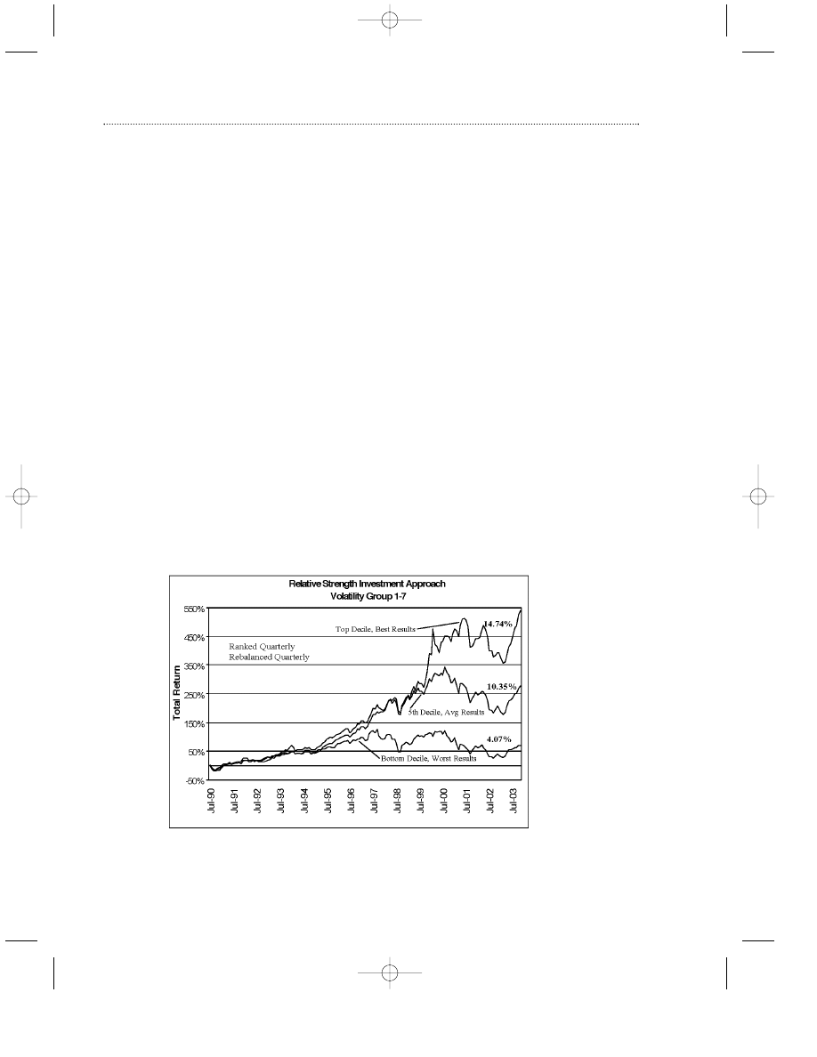
Chart 1.6

Performance of the Relative Strength Investment Approach

(1990–2003), Including Groups 6 and 7 in Addition to Groups 1–5

Appel_01T.qxd 1/26/05 8:14 PM Page 12

Rates of return for the better-performing deciles are slightly greater than rates of return for
the leading deciles in the lower-volatility Group 1–5 portfolio, but risks were clearly
increased for this higher-volatility universe of mutual funds. Returns were very consistent,
again, with decile rank: The higher the decile group was at the start of each quarter, the
better the performance.

Chart 1.6 shows the results of the study, which employs a 1–7 volatility universe

instead of a less volatile 1–5 universe. Let’s move right along to a tabular listing of
the study results.

Investment Results of Quarterly Rebalancing (June 1990–October 2003) for Mutual
Funds with Volatility Ranks 1–7 (Below to Above the S&P 500 Index)

Performance Decile

$100 Becomes

Gain Per Annum

Maximum Drawdown

First decile

$640.05

+14.7%

25.7%

Second decile

598.58

+14.2

26.1

Third decile

546.91

+13.4

27.0

Fourth decile

436.13

+11.5

33.1

Fifth decile

377.81

+10.4

37.3

Sixth decile

338.25

+9.5

39.3

Seventh decile

338.48

+9.5

39.3

Eighth decile

303.26

+8.6

39.3

Ninth decile

262.72

+7.4

38.6

Tenth decile

171.37

+4.2

44.2

The Standard & Poor’s 500 Index advanced at an annual rate of 10.8% (including
dividends) during this period, with a maximum drawdown of 44.7%.

Observations

Increasing the volatility range of the mutual fund universe from 1–5 to 1–7 resulted
in a slight improvement in the best-performing decile (+14.7 gain per annum, com-
pared to 14.1% for the lower-volatility group). However, maximum drawdowns for
the highest-performing group increased from 20.3% to 25.7%. The average gain/risk
level for the best-performing decile in the 1–5 group came to .69 (14.3% average
gain, 20.2% maximum drawdown), whereas the average gain/risk level for the best
performing decile in the 1–7 group came to .57 (14.7% average gain, 25.7% maxi-
mum drawdown).

Conclusion: There is little, if anything, to be gained in the long run by taking the

risks associated with more aggressive stock portfolios.

The No-Frills Investment Strategy

13

Appel_01T.qxd 1/26/05 8:14 PM Page 13

14

Trading Commodities and Financial Futures

Upping the Ante: The Effects of Applying the Concepts of
Relative Strength Selection to a Still More Volatile Portfolio
of Mutual Funds

Let’s try the procedure just one more time, this time with a universe of mutual
funds that includes the most volatile sectors in the equity spectrum. This universe
includes all the high-rolling areas of the stock market—gold, the internets, small
caps, technology, whatever—as well as lower-volatility funds, encompassing the
complete spectrum of mutual funds rated by volatility as 1–9.

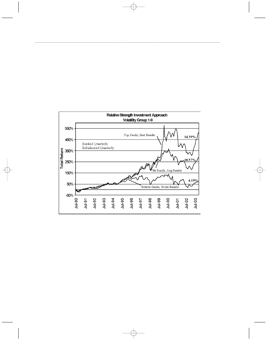
Chart 1.7

Performance of the Relative Strength Investment Approach (1990–2003),

Including All Mutual Fund Groups, Rated as 1–9

Rates of return for the best deciles in the 1–9 universe remained in the area of returns secured
from lower-volatility mutual fund universes 1–5 and 1–7. However, risks increased considerably,
as you can see by the drawdowns reflected on the chart. The first-performance decile for the
previous quarter proved, again, to be the best for the subsequent quarter, although the lead
over the second-best-performing decile the previous quarter was not great.

Appel_01T.qxd 1/26/05 8:14 PM Page 14

Let’s review, just one more time, a tabular table.

Investment Results of Quarterly Rebalancing (June 1990–October 2003)
Mutual Funds with Volatility Ranks 1–9 (Virtually All Equity-Oriented Mutual
Funds, Including Those Considerably More Volatile Than the Standard & Poor’s
500 Index

Performance Decile

$100 Becomes

Gain Per Annum

Maximum Drawdown

First decile

$596.31

+14.1%

20.3%

First decile

$614.44

+14.3%

40.2%

Second decile

605.24

+14.3

34.2

Third decile

539.98

+13.3

31.5

Fourth decile

454.66

+11.9

38.6

Fifth decile

388.29

+10.6

39.9

Sixth decile

335.07

+9.4

41.8

Seventh decile

330.19

+9.3

42.2

Eighth decile

296.95

+8.4

43.7

Ninth decile

267.68

+7.6

43.1

Tenth decile

173.97

+4.2

50.1

General Observations

Again, we see a very linear relationship between fund performance in a previous
quarter and its performance in subsequent periods. Within the highest-velocity
mutual fund group, the second decile runs very closely in strength to the first decile.
I have found this to be the case in studies I have conducted of other ways to employ
past relative strength to predict future market performance. It seems that, among the
most volatile mutual fund areas, more consistent performance is sometimes attained
from second and third decile holdings than by first, although, in this study, the first
decile produced the best rates of return.

The average gain/maximum drawdown ratio for even the strongest (first decile)

area of the 1–9 group of mutual funds is low, at 0.36 (14.39 rate of return, 40.18%
maximum drawdown). The gains can be there, but the pains can be considerable,
indeed, for investors who live in the fast lane.

Although portfolios are rebalanced at quarterly intervals, this does not mean that

you will have to replace your entire portfolio each quarter. On average, holdings are
likely to be maintained through two quarterly cycles, or for six months in total.
Conclusion: Increasing the volatility of your mutual fund portfolio does not add to
profitability in any significant manner, even though risk levels do increase. As a gen-
eral rule, your emphasis should remain with funds of average or below-average
volatility.

The No-Frills Investment Strategy

15

Appel_01T.qxd 1/26/05 8:14 PM Page 15

16

Trading Commodities and Financial Futures

A Quick Review of Relative Strength Investing

The three-step procedure for managing your mutual fund portfolio:

Step 1: Secure access to data sources that will provide you with at least
quarterly price data and volatility ratings of a universe of at least
500 (preferably somewhat more) mutual funds. (Suggestions have
been provided.)

Step 2: Open an investment account with a diversified portfolio of mutual
funds whose performance the previous quarter lay in the top 10% of the
mutual funds in your trading universe and whose volatility is equal to or less
than the Standard & Poor’s 500 Index, or, at the most, no greater than the
average fund in your total universe.

Step 3: At the start of each new quarter, eliminate those funds in
your portfolio that have fallen from the first performance decile,
replacing them with funds that are currently in the top performance
decile.

This account is probably best carried forth at a brokerage house that provides a
broad platform of mutual funds into which investments may be placed. Schwab and
T. D. Waterhouse, for example, provide both the requisite service and the requisite
mutual fund platform. Other brokerage firms might do so as well.

Summing Up

To sum up, we have reviewed a strategy for maintaining mutual fund portfolios that
has been effective since at least 1990 (almost certainly longer), a strategy that pro-
duces returns that well exceed buy-and-hold strategies while significantly reducing
risk.

These strategies appear to be effective with a variety of investments, including

mutual funds, ETFs, and probably (although I have not personally tested for this)
individual stocks as well. Generally, mutual funds seem somewhat more suited for
this approach than ETFs, which tend, on average, to be more volatile than the best-
performing mutual fund universe (1–5).

You have learned a significant strategy for outperforming buy-and-hold strate-

gies in the stock market, a strategy based upon relative-strength mutual fund selec-
tion, not upon market timing.

Let’s move along to the next chapter and to two simply maintained indicators

that can help you decide when to buy.

Appel_01T.qxd 1/26/05 8:14 PM Page 16