Badania operacyjne (część 3)
Zagadnienie optymalizacji
Programowanie liniowe
Programowanie w liczbach całkowitych
Programowanie nieliniowe.
Zagadnienie optymalizacyjne
Funkcja celu (kryterium decyzyjne)
f(x) = f(x1, x2, … , xn)
Zmienne decyzyjne (wielkości optymalizowane)
xj (j=1, 2, … , n)
Ograniczenia, warunki ograniczające (funkcja nakładów)
Vi(x) = Vi(x1, x2, … , xn) (i=1, 2, … , m) (warunki uboczne).
Funkcje celu i nakładów są ciągłe i różniczkowalne (posiadają ciągłe pochodne cząstkowe pierwszego i drugiego rzędu) i są określone na n-wymiarowym wektorze x o nieujemnych składowych
(warunki brzegowe)
czyli
(j=1, 2, … , n).
Zadanie optymalizacyjne polega na wyznaczeniu ekstremum (maksimum lub minimum) funkcji celu przy zadanych ograniczeniach.
Zadanie optymalizacyjne ma rozwiązanie jeśli nie jest wewnętrznie sprzeczne (zbiór rozwiązań dopuszczalnych nie jest zbiorem pustym) oraz gdy
.
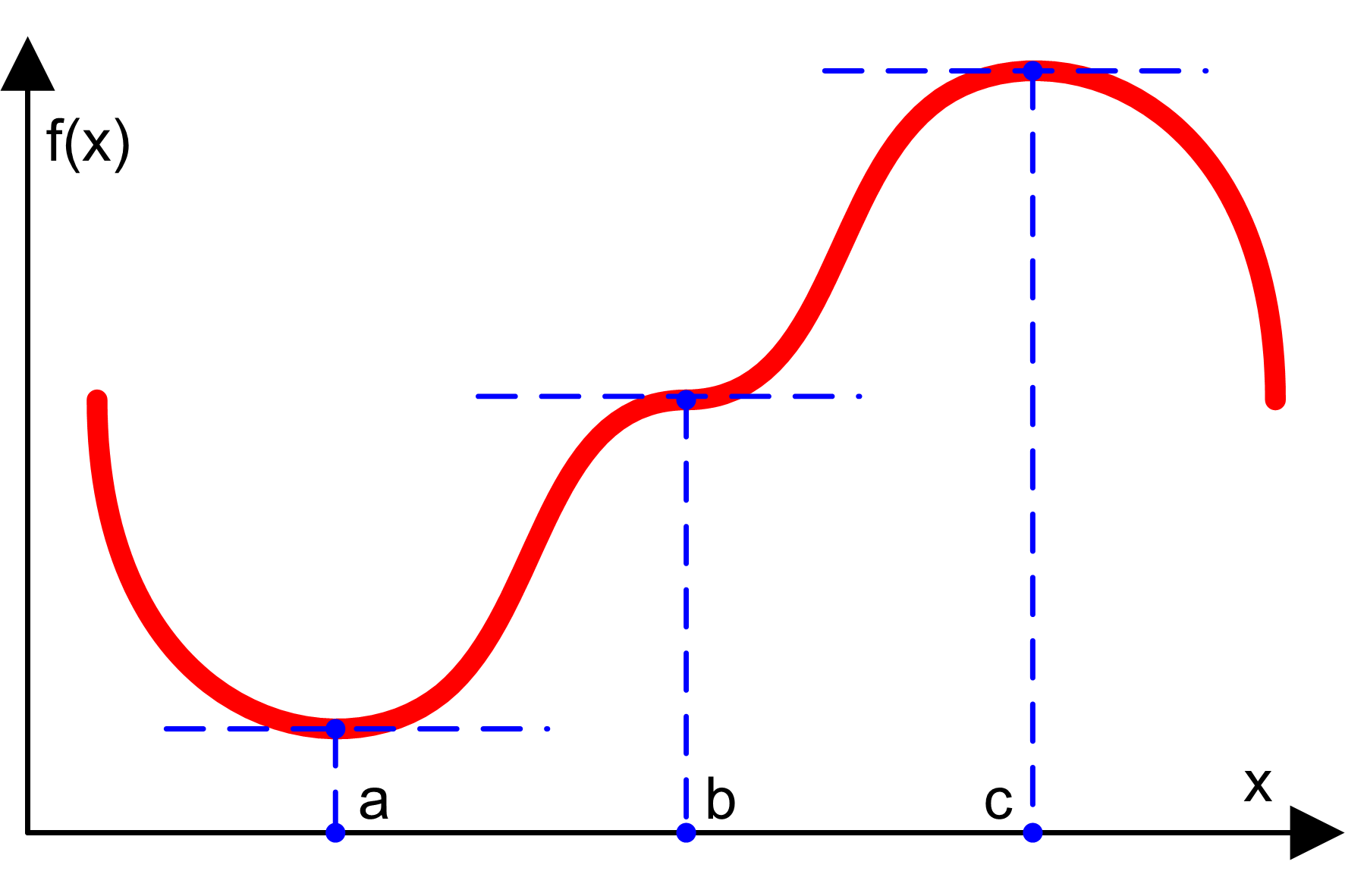
Ekstremum funkcji jednej zmiennej
Funkcja celu: f(x)
W przedziale istnieje taki punkt x0, że f'(x0)=0 oraz f''(x0)
0Druga pochodna f''(x0) jest ciągła - w punkcie x0 istnieje ekstremum:
maksimum jeśli f''(x0)<0
minimum jeśli f''(x0)>0.
Dla f''(x0)=0 w punkcie x0 istnieje punkt przegięcia.
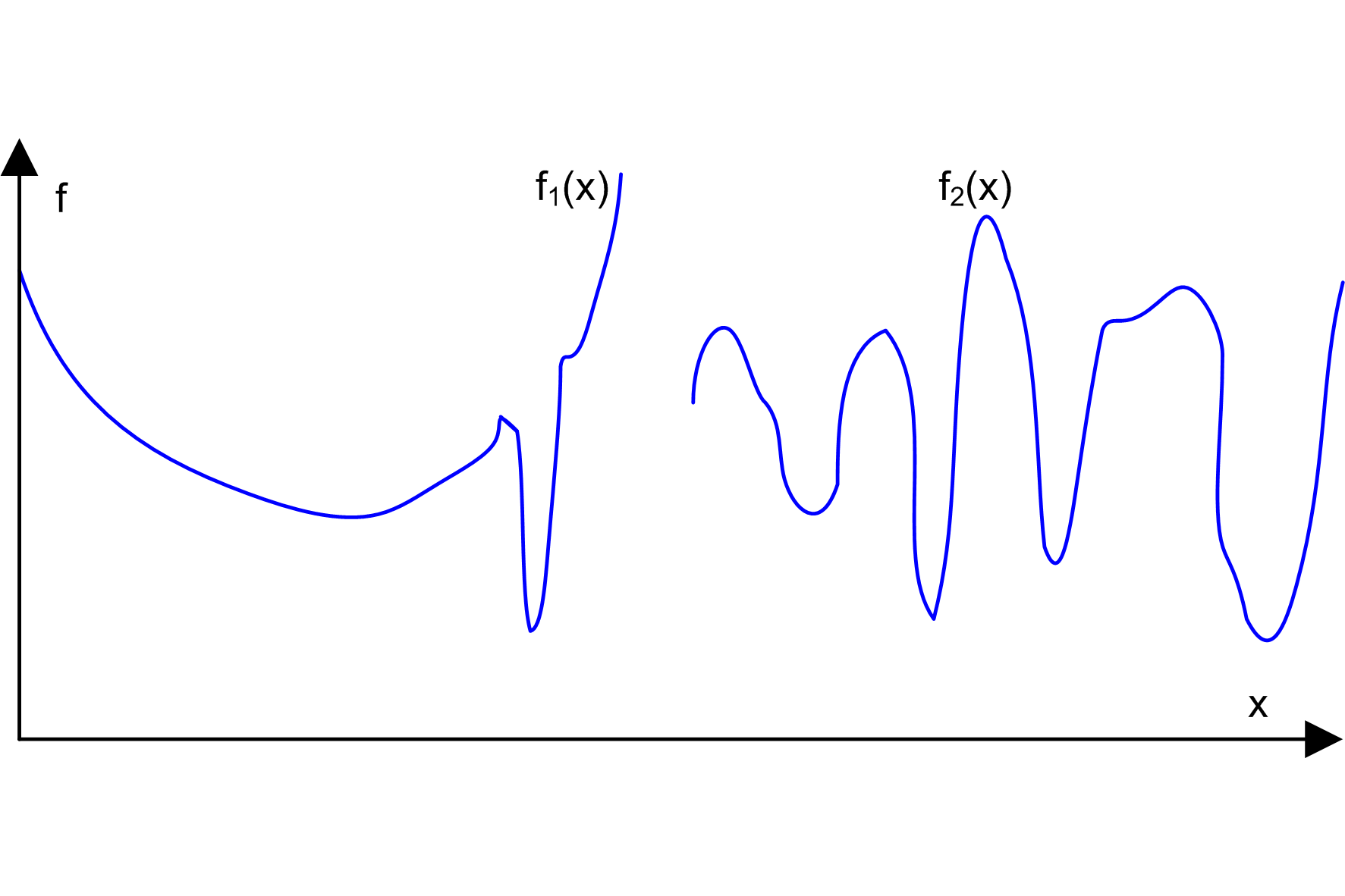
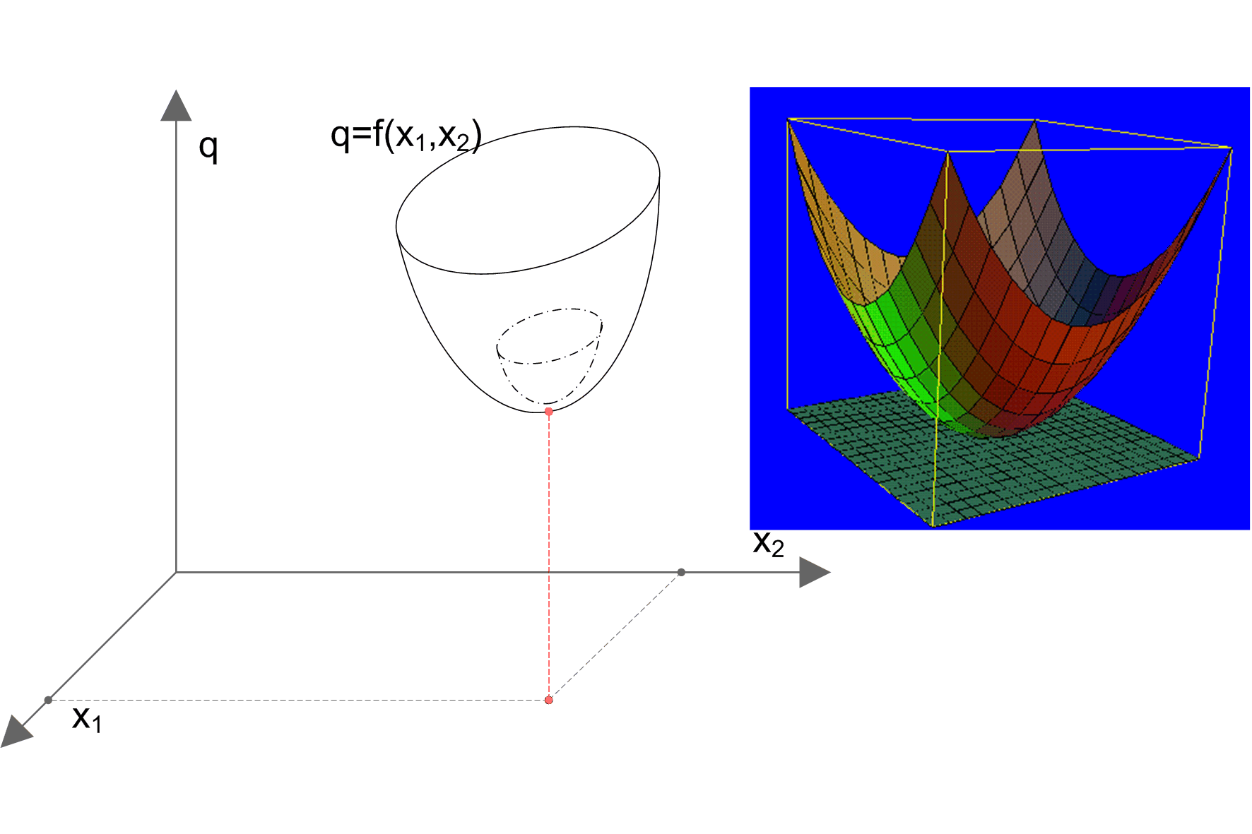
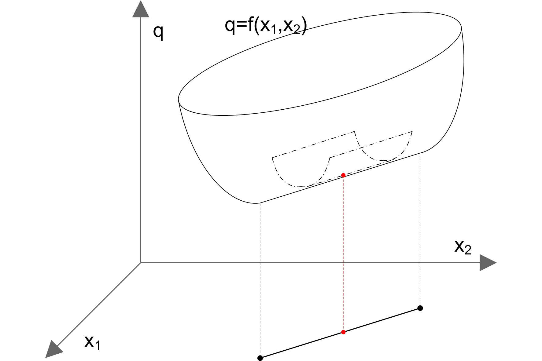
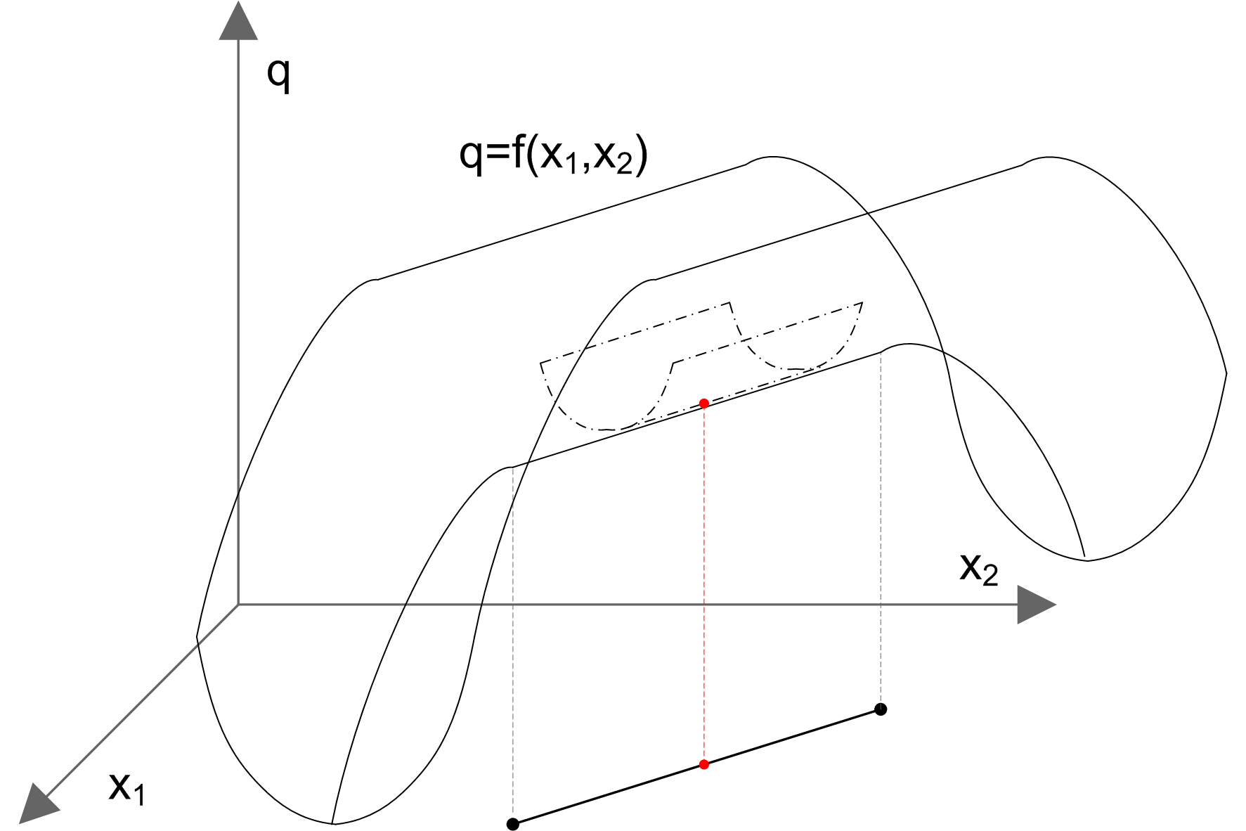
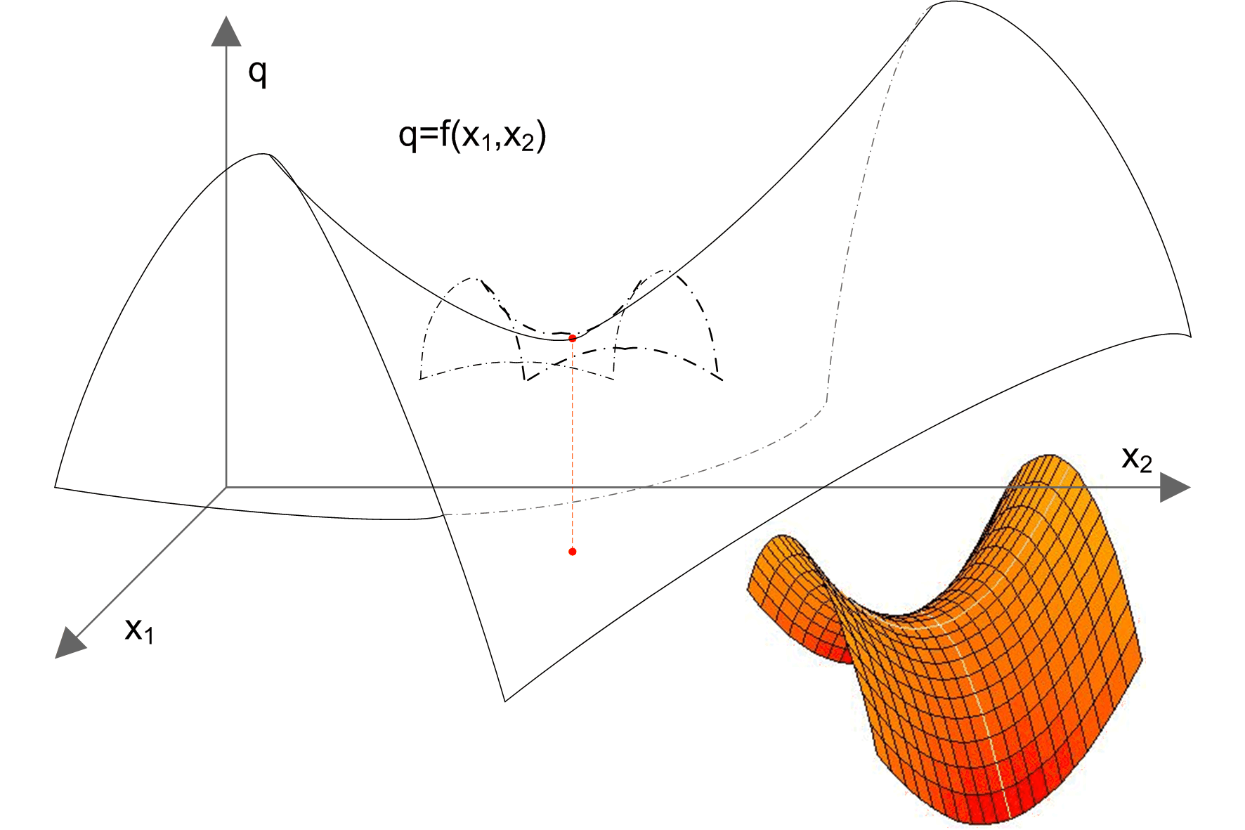
Funkcje trudne do optymalizacji
Ekstremum funkcji n zmiennych
Funkcja celu - f(x)
Hesjan funkcji f(x) w punkcie x=(x1, x2, … xn)
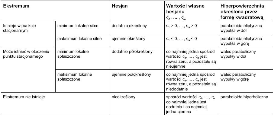
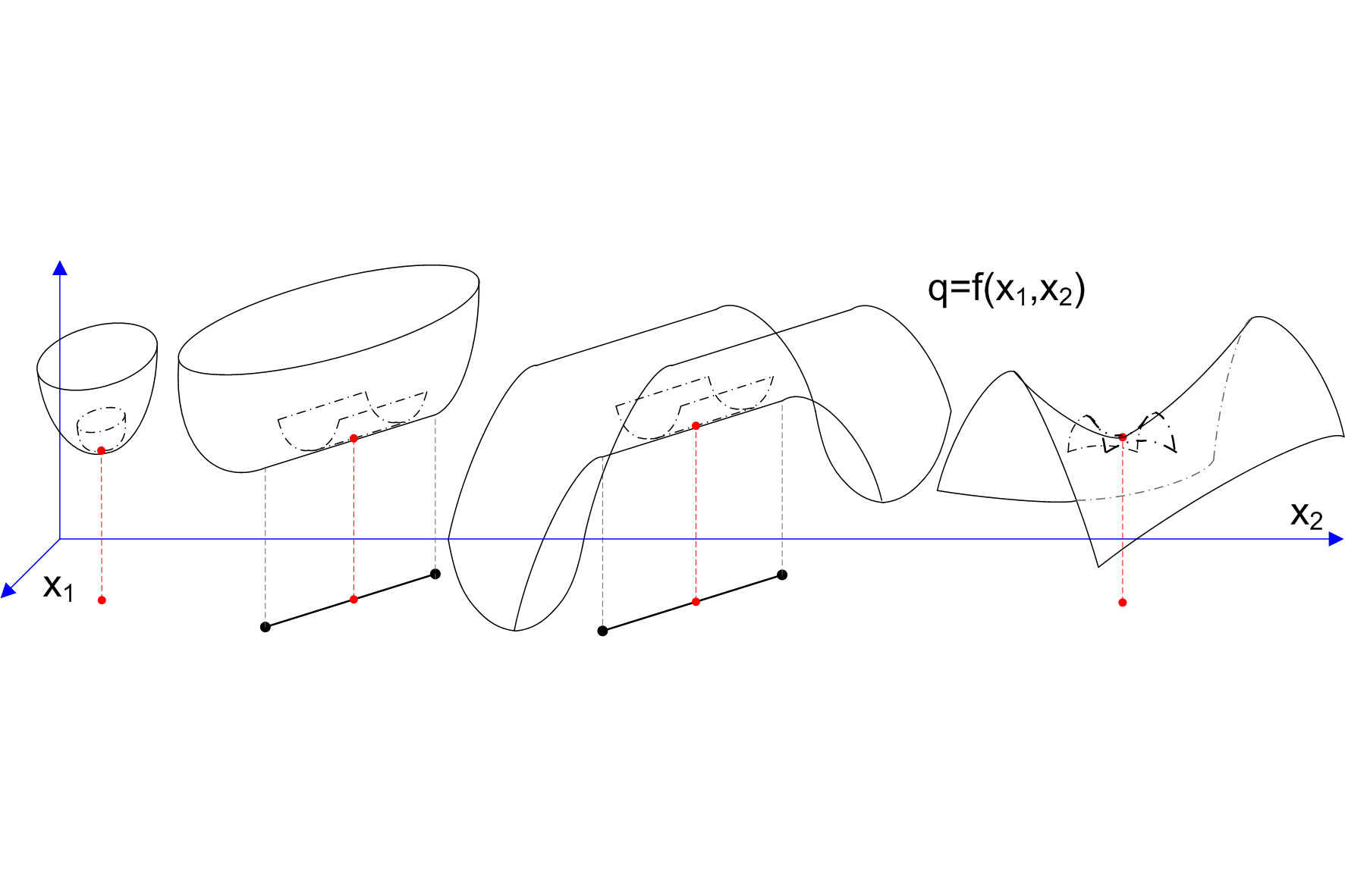
Paraboloida eliptyczna wypukła w dół
Walec paraboliczny wypukły w dół
Minimum spłaszczone
Walec paraboliczny wypukły w dół
Minimum spłaszczone nie istnieje
Paraboloida hiperboliczna
Programowanie liniowe
Programowanie liniowe (ang: linear programming) - liniowe zagadnienie optymalizacji.
Zagadnienia optymalizacji były rozwijane niezależnie w różnych dziedzinach nauki, stąd terminologia poszczególnych zagadnień jest zróżnicowana i niespójna. Spowodowało to powstanie i upowszechnienie wielu specyficznych określeń, takich jak - `programowanie liniowe', `programowanie nieliniowe'.
Określenia te posiadają długą tradycję, stąd w niektórych dziedzinach (np. ekonomii) są powszechnie używane. Jednak w naukach technicznych są uznawane za wybitnie mylące, ze względu na skojarzenia z programowaniem komputerów. Dlatego w teorii optymalizacji używa się określenia `poszukiwanie ekstremum funkcji liniowych przy liniowych warunkach ograniczających'.
Funkcja celu jest:
funkcją liniową - zawiera zmienne decyzyjne wyłącznie stopnia pierwszego
(np. f(x1) = a*x1+ b)
lub jest formą liniową - funkcją liniową bez wyrazu wolnego od zmiennej x1
(np. f(x1) = a*x1)
Warunki uboczne Vi(x) = Vi(x1, x2, … , xn) (i=1, 2, … , m) mają postać układu równań liniowych
ai1x1 + ai2x2 + … + ainxn = bi (i=1, 2, … , m)
lub nierówności liniowych
ai1x1 + ai2x2 + … + ainxn ˇÂ bi (i=1, 2, … , m)
Warunki uboczne oraz brzegowe wyznaczają dopuszczalny obszar rozwiązań.
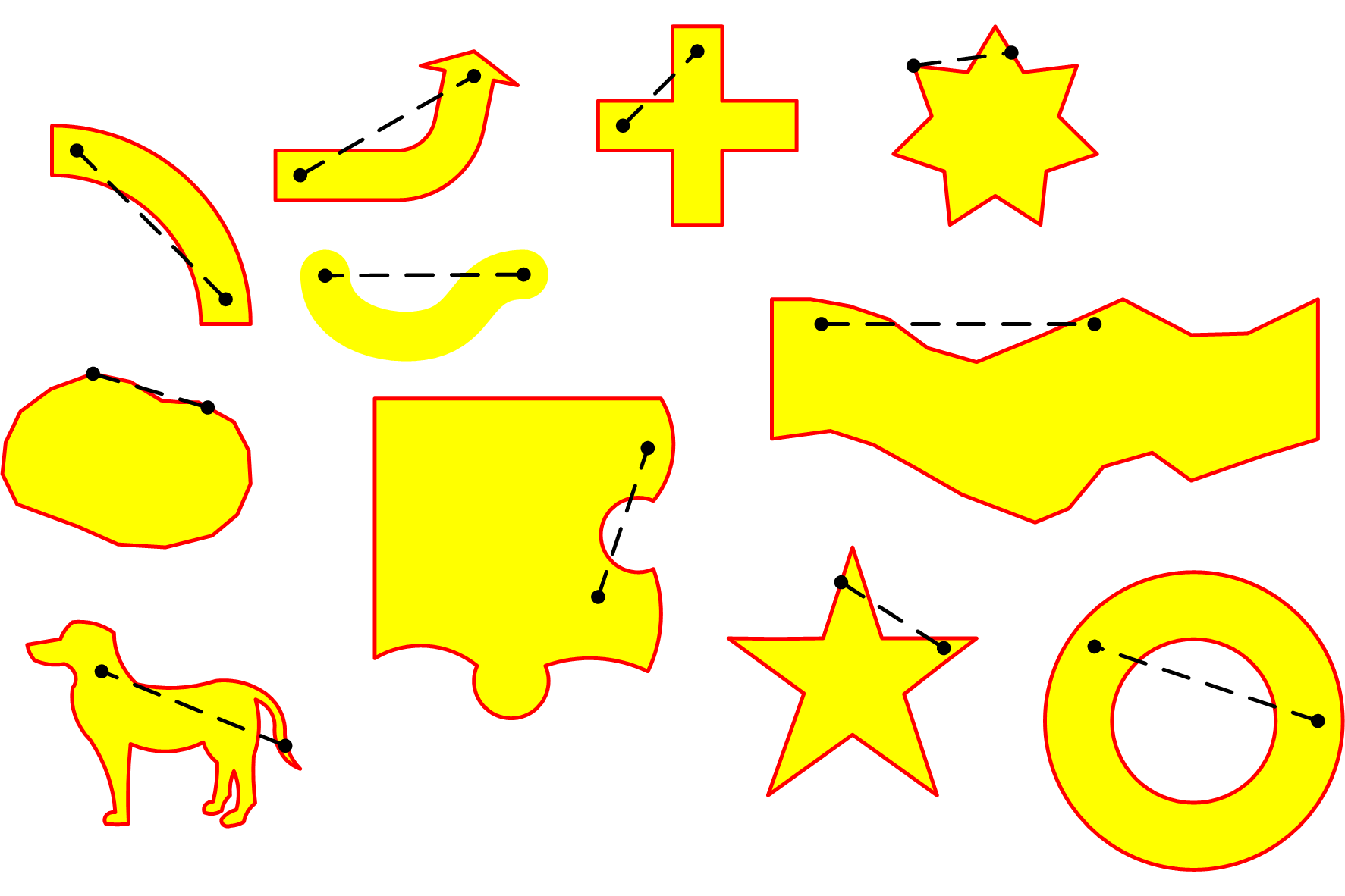
Zbiór wypukły
Zbiór punktów, dla którego wszystkie punkty na odcinku łączącym dwa punkty p i q należące do zbioru - należą również do tego zbioru.
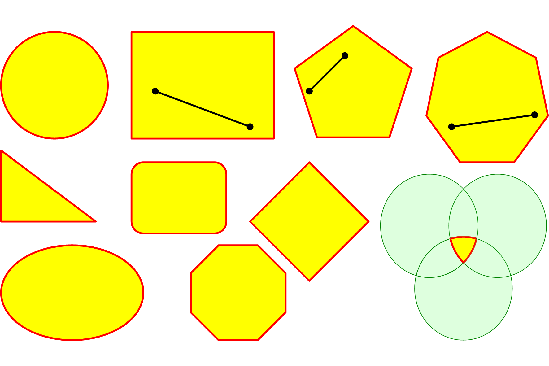
Zbiory niewypukłe
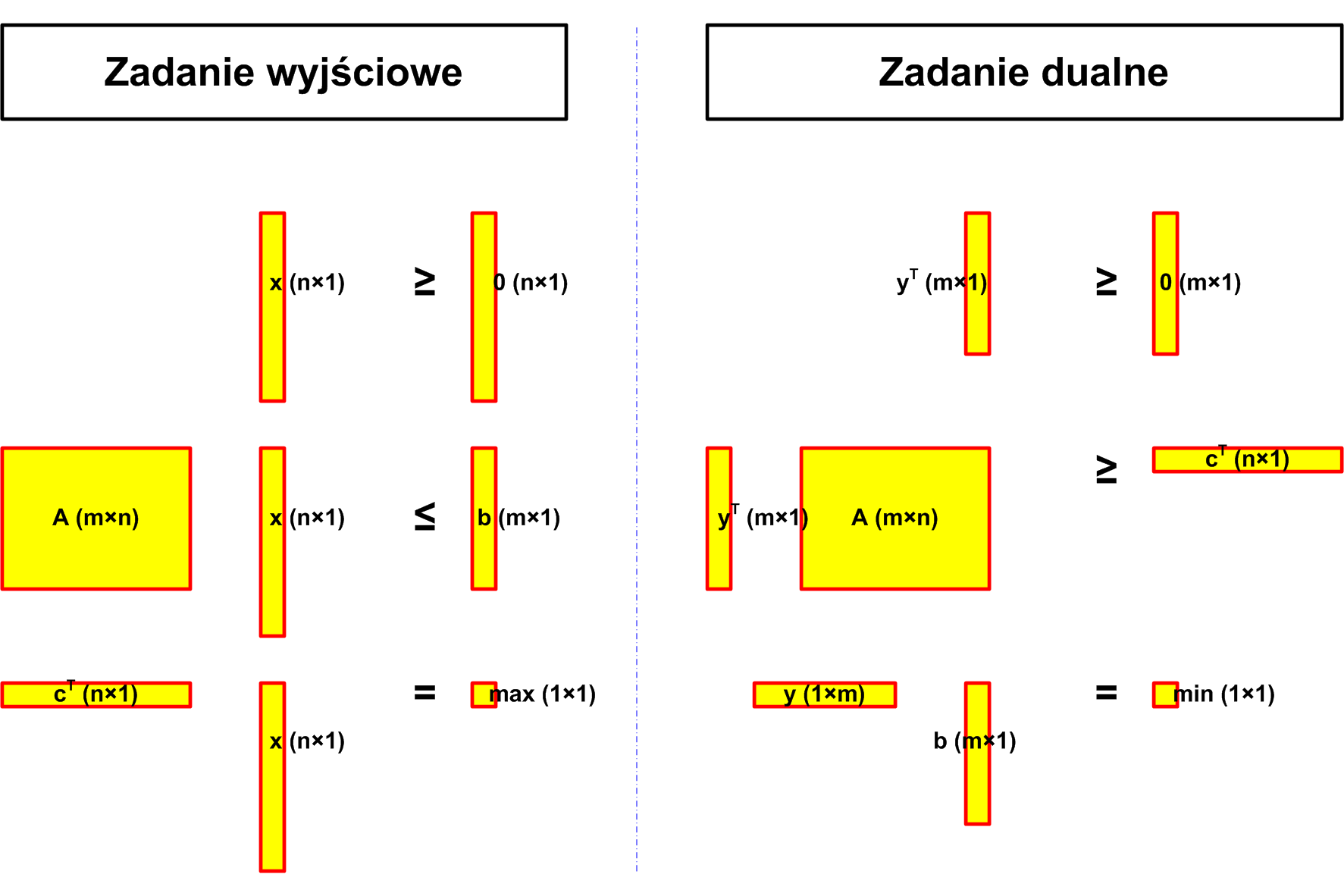
Zagadnienie dualne programowania liniowego
Pierwotne zadanie wyjściowe
cT x
max,
A x
b,
x
0.
Dla każdego zagadnienia programowania liniowego można stworzyć dualne zagadnienie, które również jest zagadnieniem programowania liniowego. Między zagadnieniami występują wzajemne zależności - np. zadanie dualne zagadnienia dualnego jest wyjściowym zadaniem pierwotnym.
Zadanie dualne
y b
min,
yT A
cT,
yT
0.
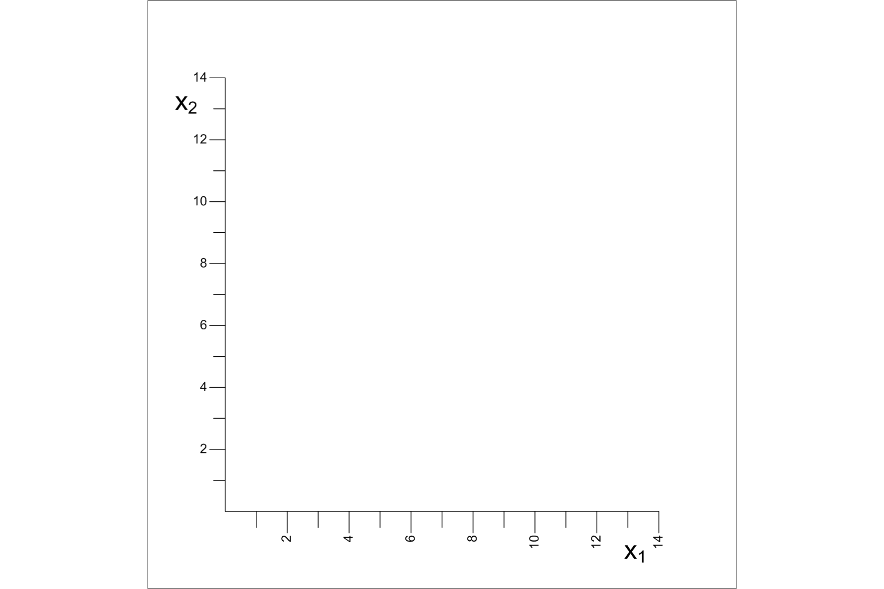
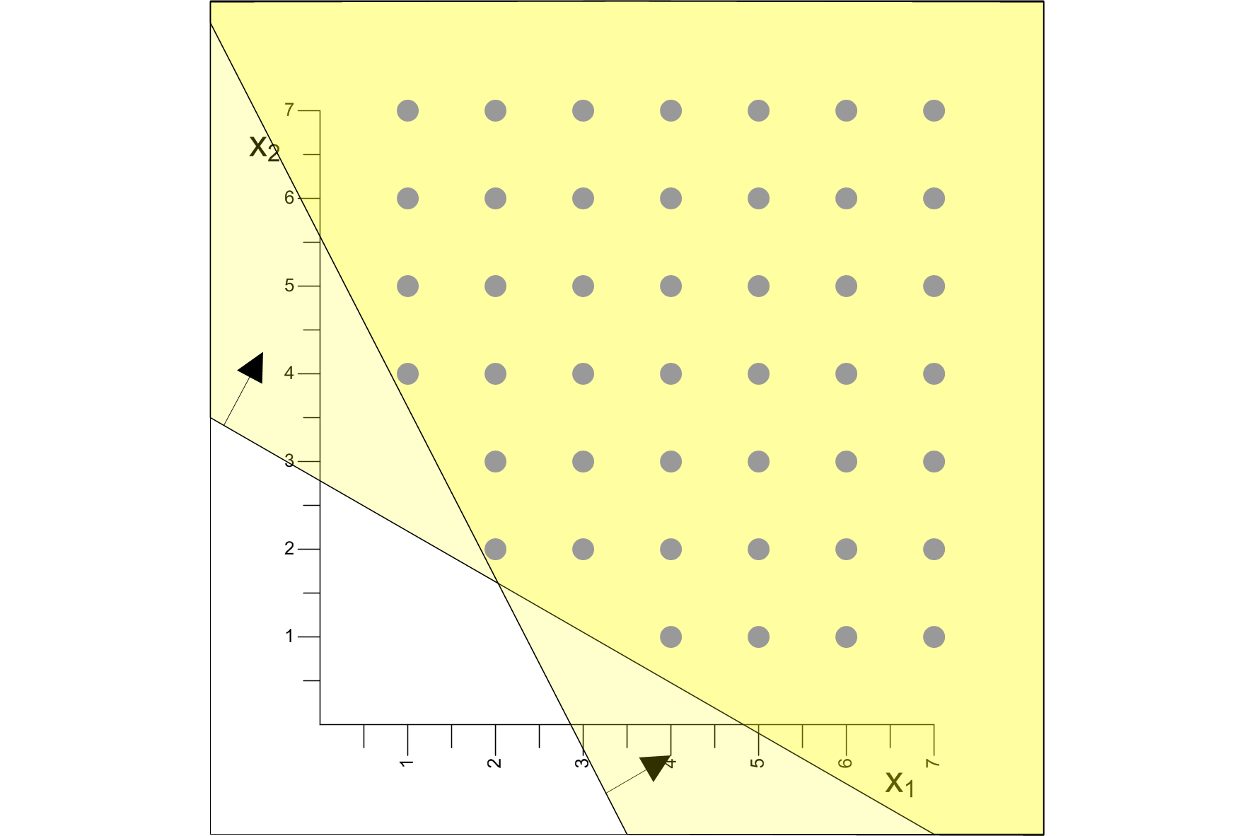
Przykład: planowanie produkcji
Przedsiębiorstwo może produkować dwa wyroby:
X1 - urządzenie o opanowanej technologicznie produkcji, choć niezbyt nowoczesne,
X2 - urządzenie nowoczesne, jednak o wyższych kosztach komponentów i mniejszej zyskowności produkcji.
Rozpatrywane zagadnienie polega na określeniu optymalnej wielkości produkcji obu wyrobów, przynoszącej przedsiębiorstwu maksymalny zysk.
Zmienne decyzyjne:
x1 - wielkość produkcji wyrobu X1,
x2 - wielkość produkcji wyrobu X2.
Swobodę decyzyjną ograniczają zasoby przedsiębiorstwa:
99 jednostek surowca,
96 jednostek czasu pracy urządzeń produkcyjnych,
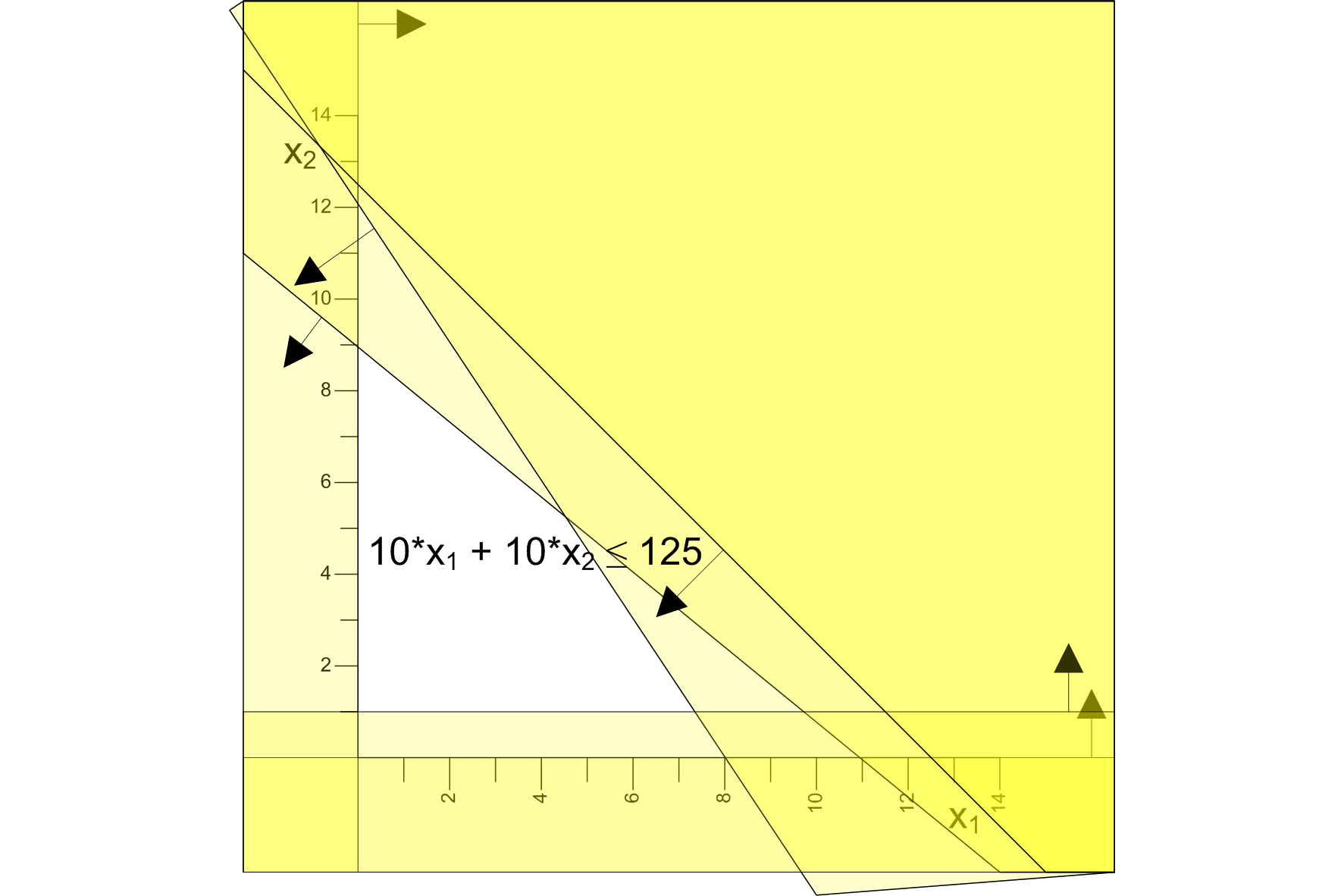
125 jednostek powierzchni produkcyjnej,
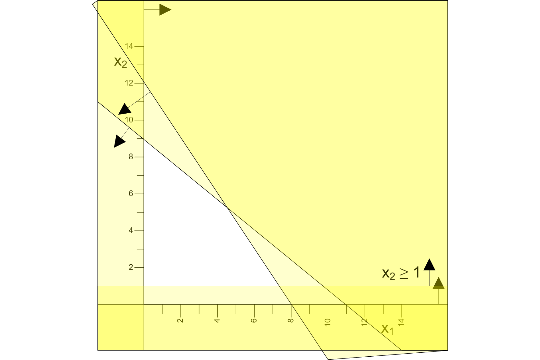
utrzymanie się na rynku branży wymaga wyprodukowania co najmniej 1 jednostki (partii) wyrobu X2.
Jednostkowe zużycie zasobów (spowodowane stosowanymi technologiami) wymaga:
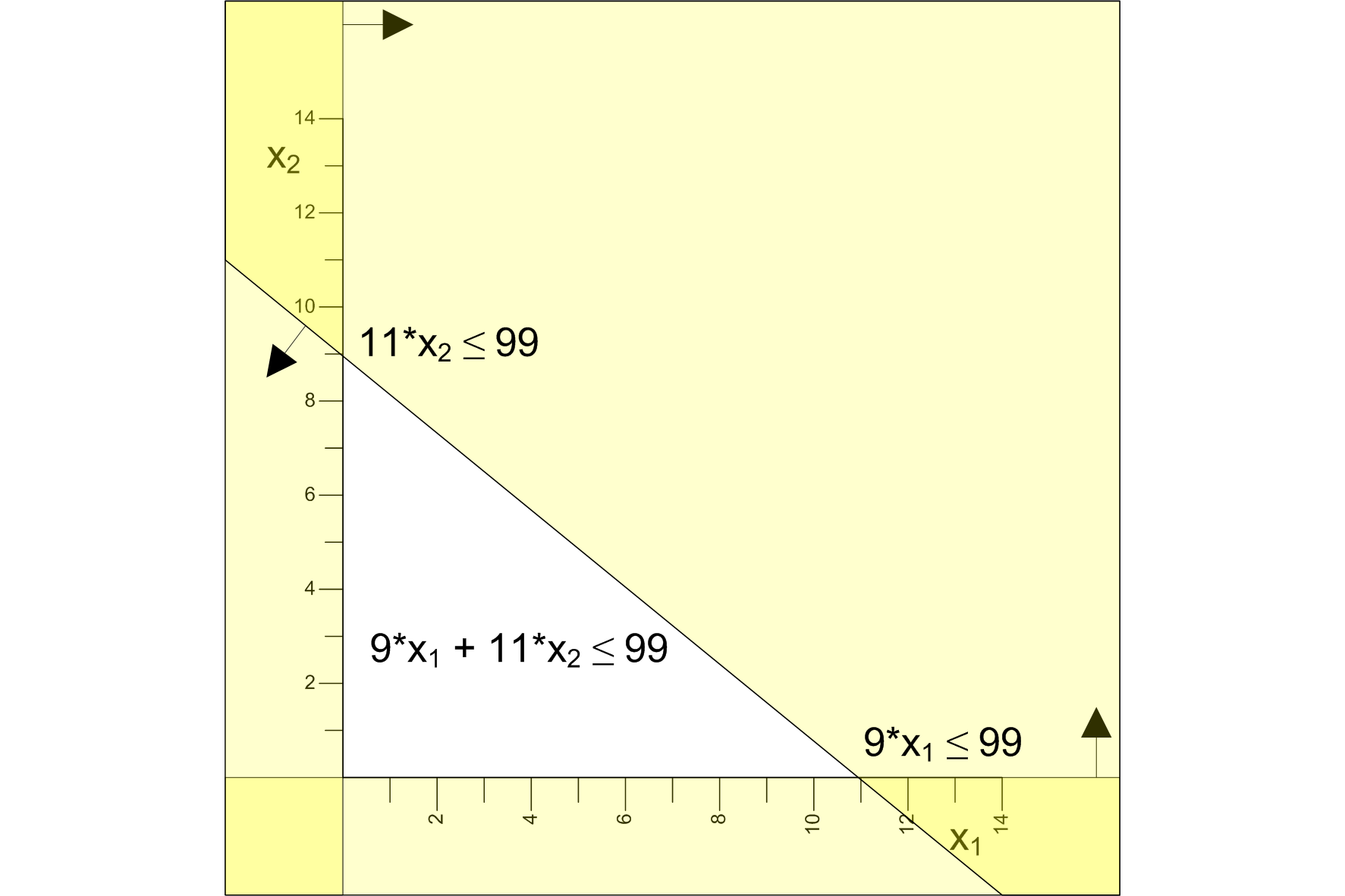
zużycia surowców -
9 jednostek surowca na jednostkę wyrobu X1,
11 jednostek surowca na jednostkę X2.
czasu pracy urządzeń -
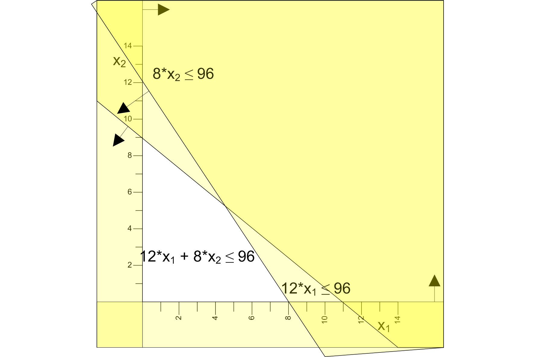
12 jednostek czasu pracy na jednostkę wyrobu X1,
8 jednostek czasu na jednostkę X2.
wykorzystania powierzchni produkcyjnej -
10 jednostek powierzchni na jednostkę wyrobu X1,
10 jednostek powierzchni na jednostkę X2.
Jednostkowe zyski z produkcji wynoszą odpowiednio:
6 jednostek monetarnych na jednostkę wyrobu X1,
2.5 jednostek monetarnych na jednostkę X2.
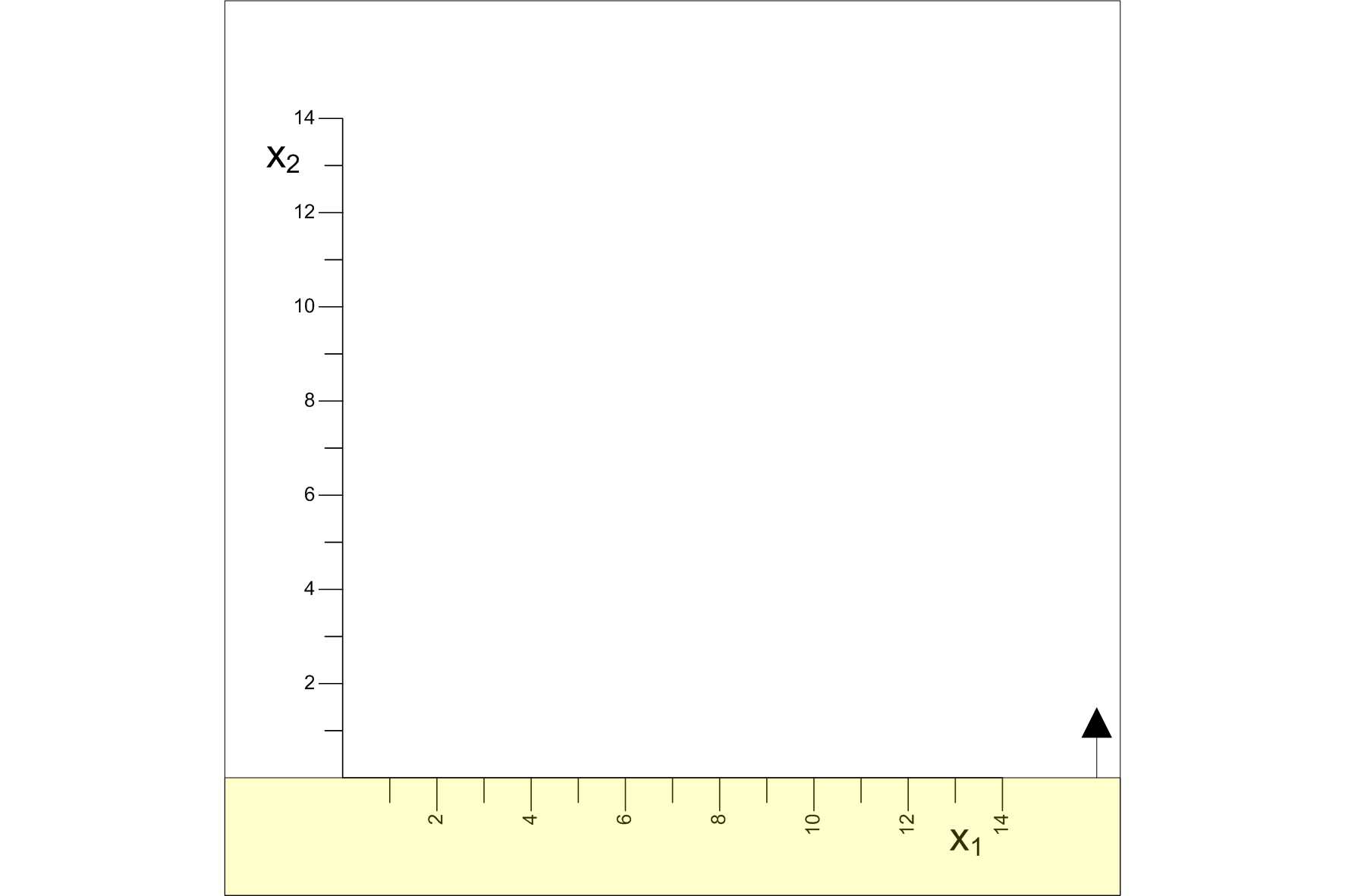
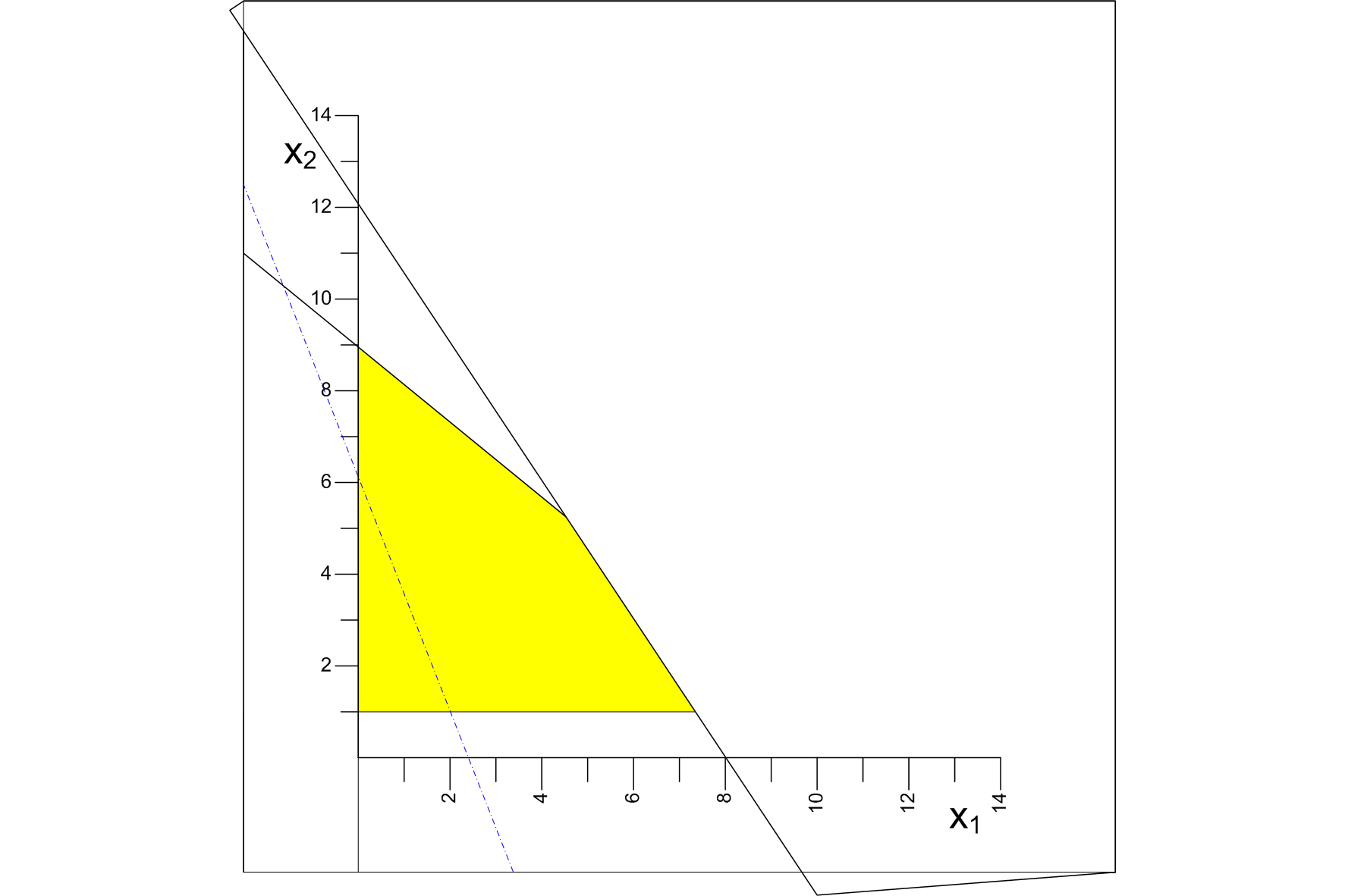
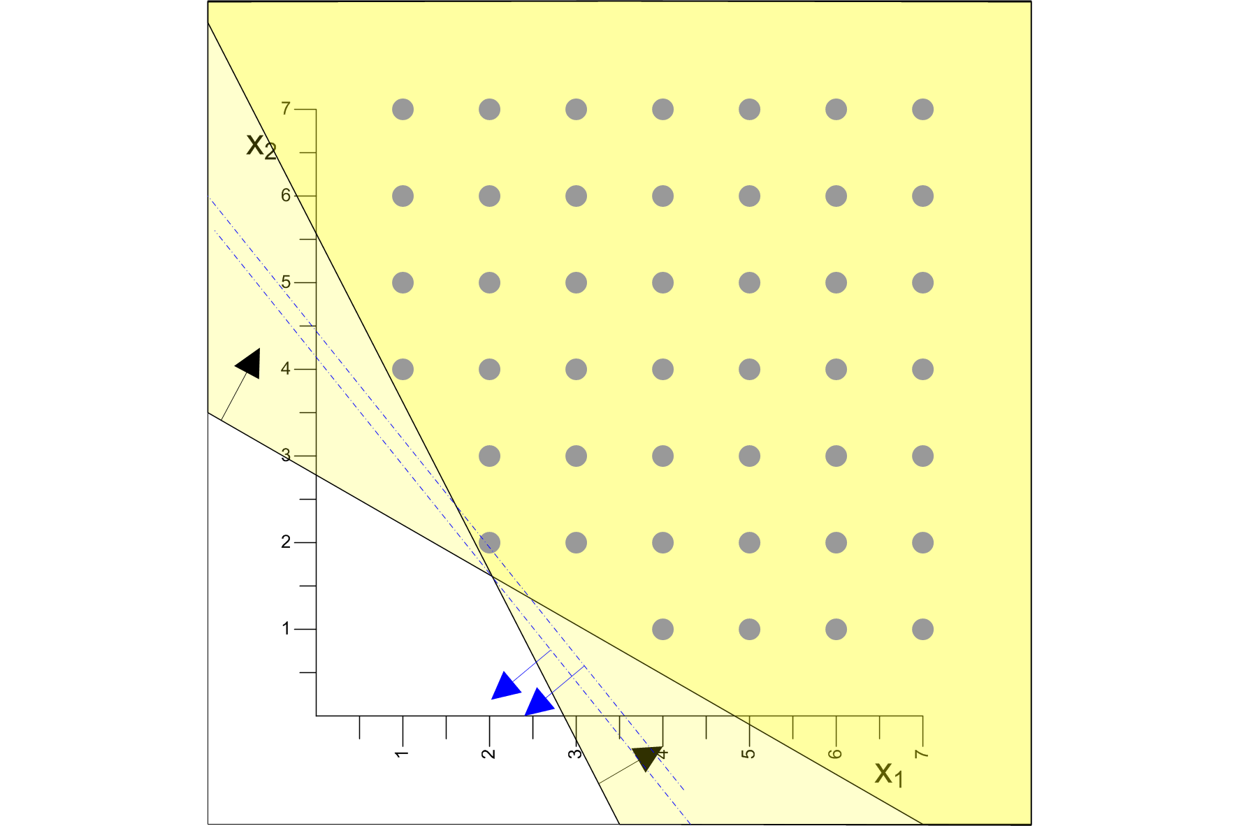
Model matematyczny zagadnienia:
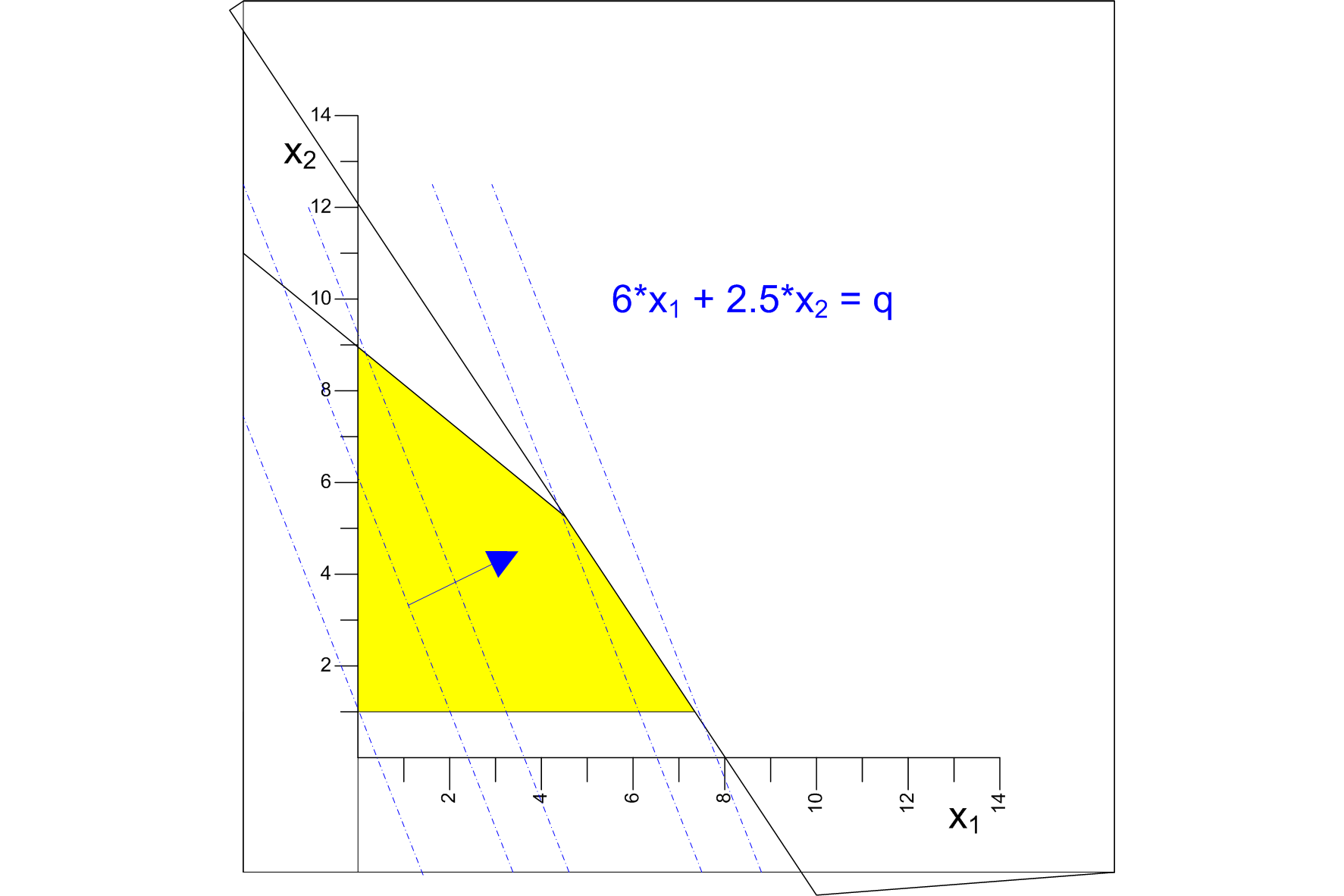
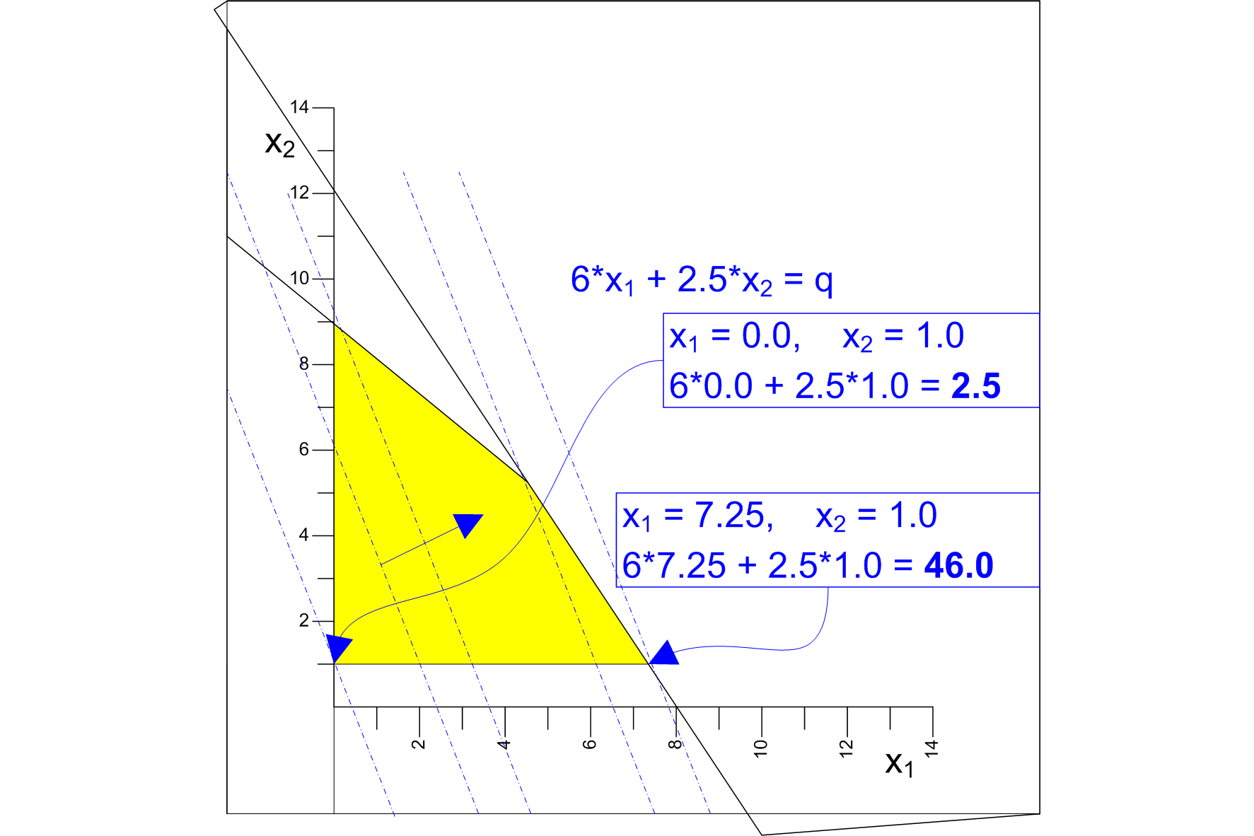
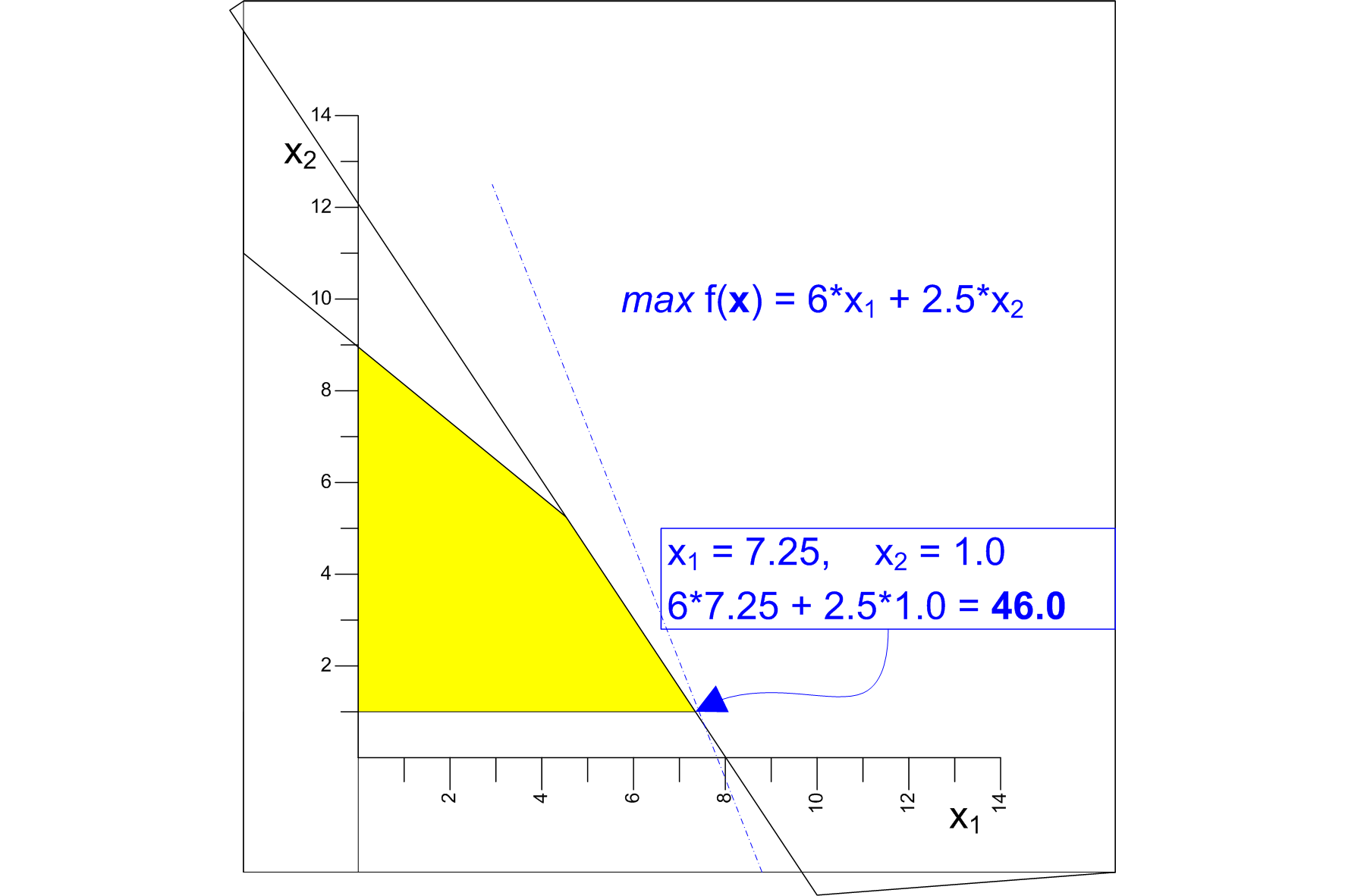
max f(x) = 6*x1 + 2.5*x2 (zysk z produkcji)
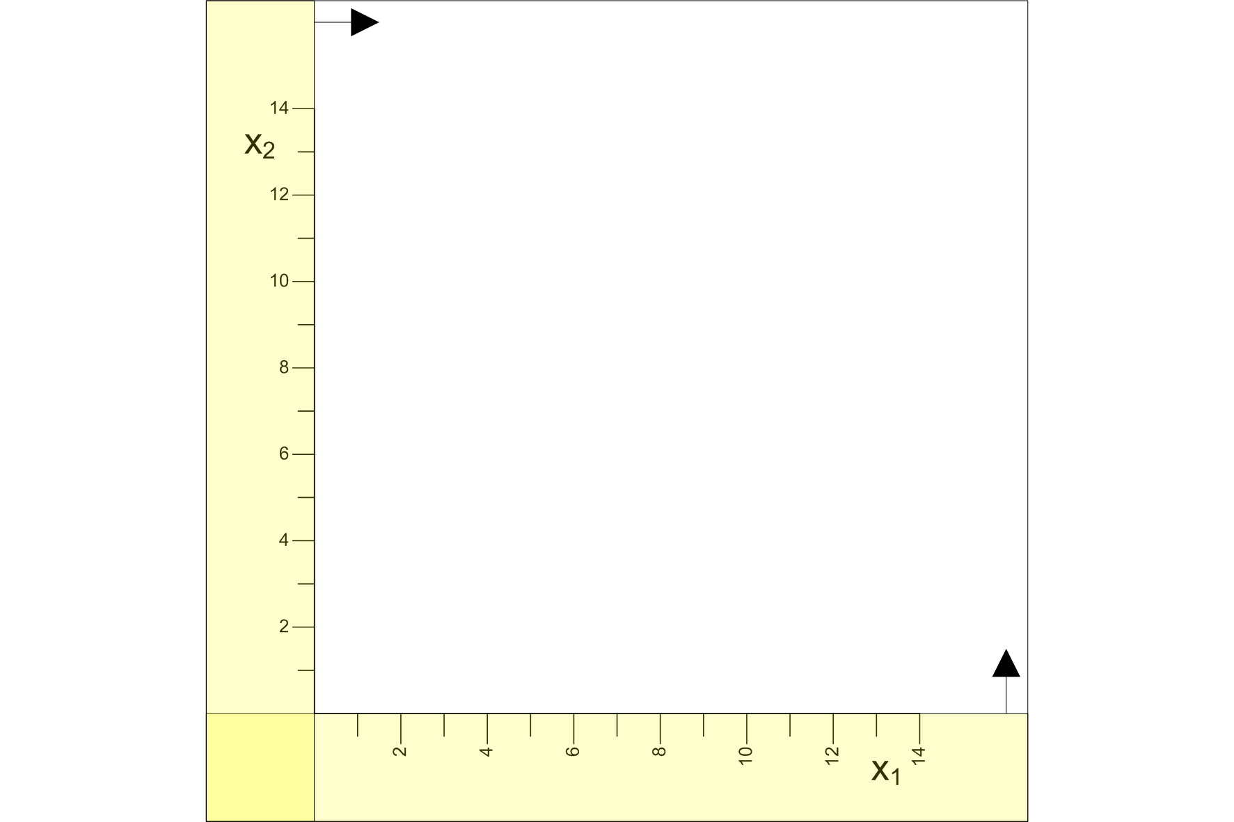
x1
0
x2
0
9*x1 + 11*x2
99 (zużycie surowców)
12*x1 + 8*x2
96 (wykorzystanie urządzeń)
x2
1 (warunek utrzymania się na rynku)
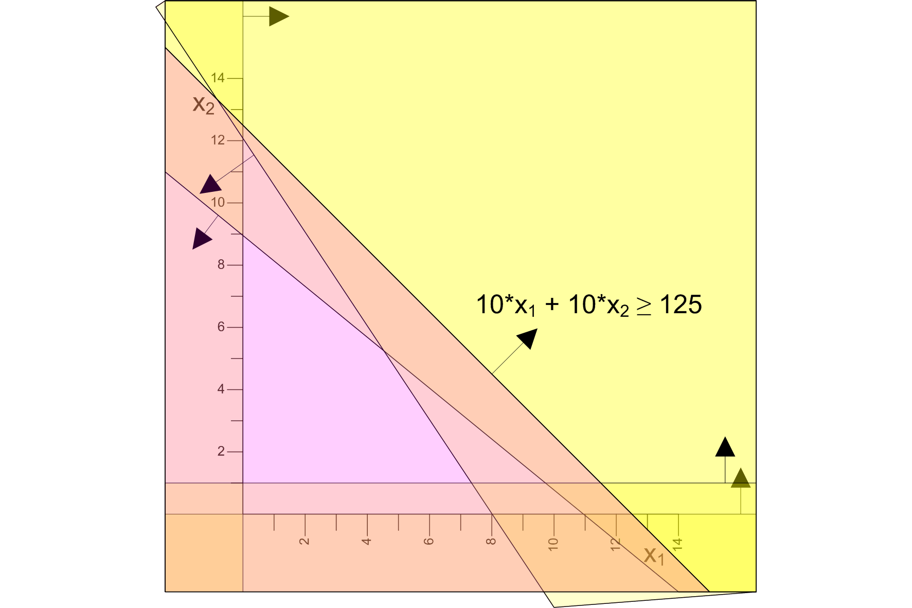
10*x1 + 10*x2
125 (powierzchnia produkcyjna)


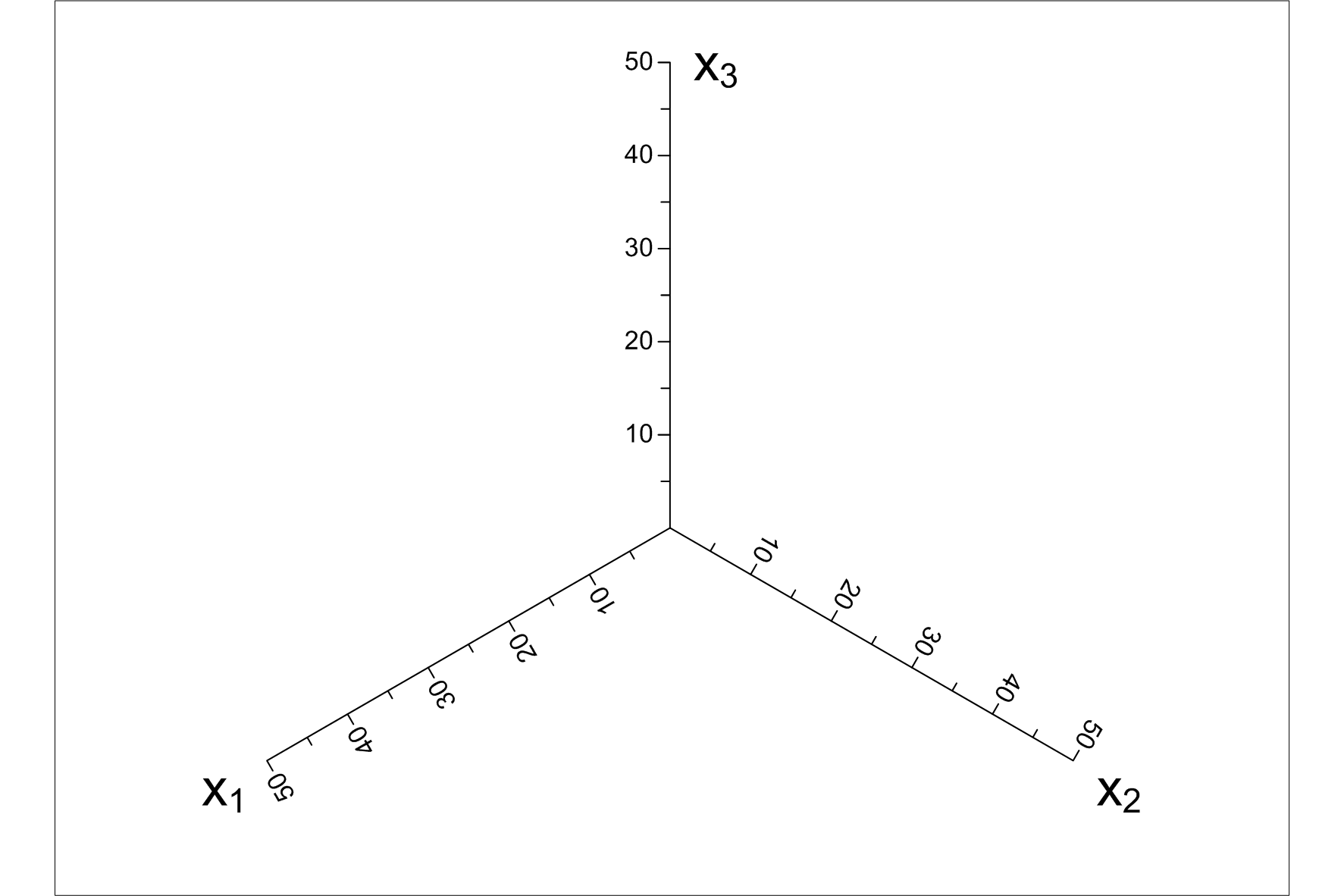
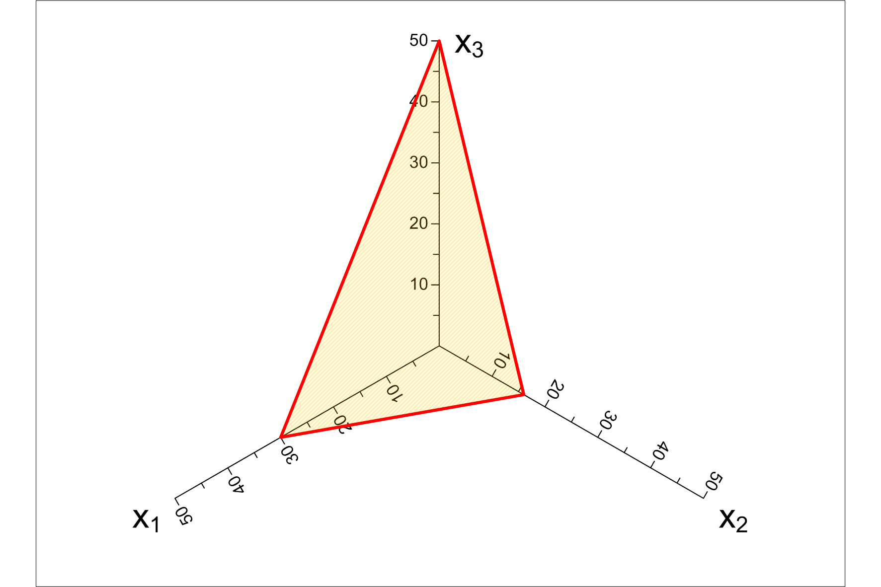
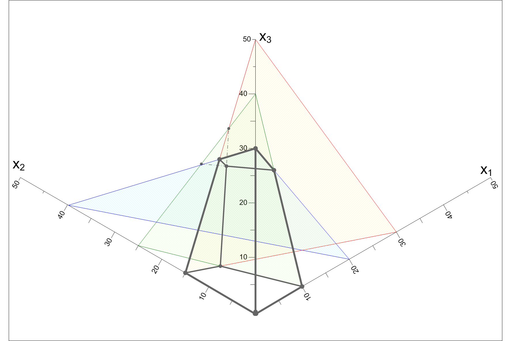
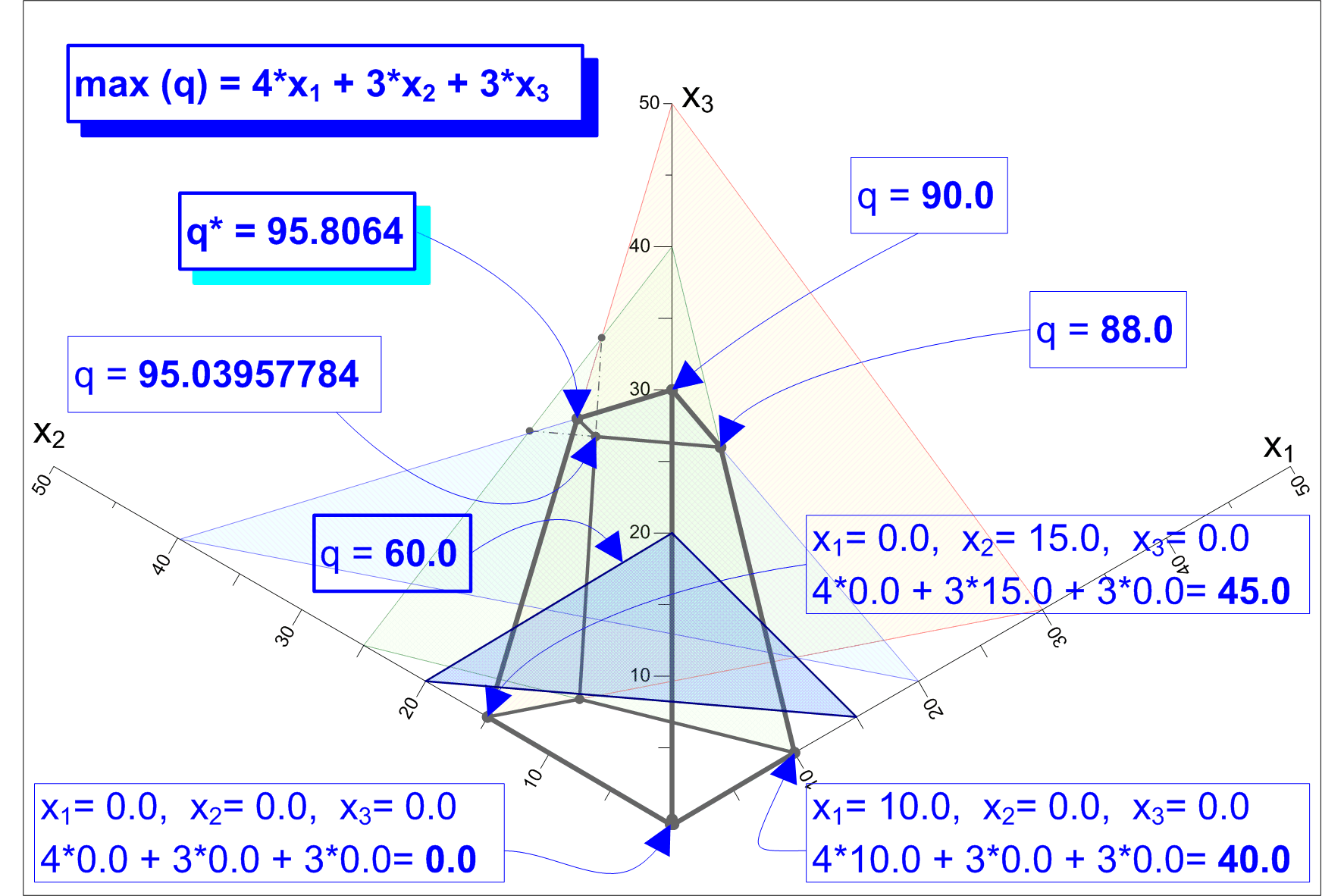
Zagadnienie trójwymiarowe
Model matematyczny zagadnienia:
max f(x) = 4*x1 + 3*x2 + 3*x3
75*x1 + 150*x2 + 45*x3
2250
120*x1 + 60*x2 + 80*x3
2400
100*x1 + 40*x2 + 25*x3
1000
x1
0, x2
0, x3
0
Aksonometria `kawaleryjska' - identyczna skala na wszystkich osiach
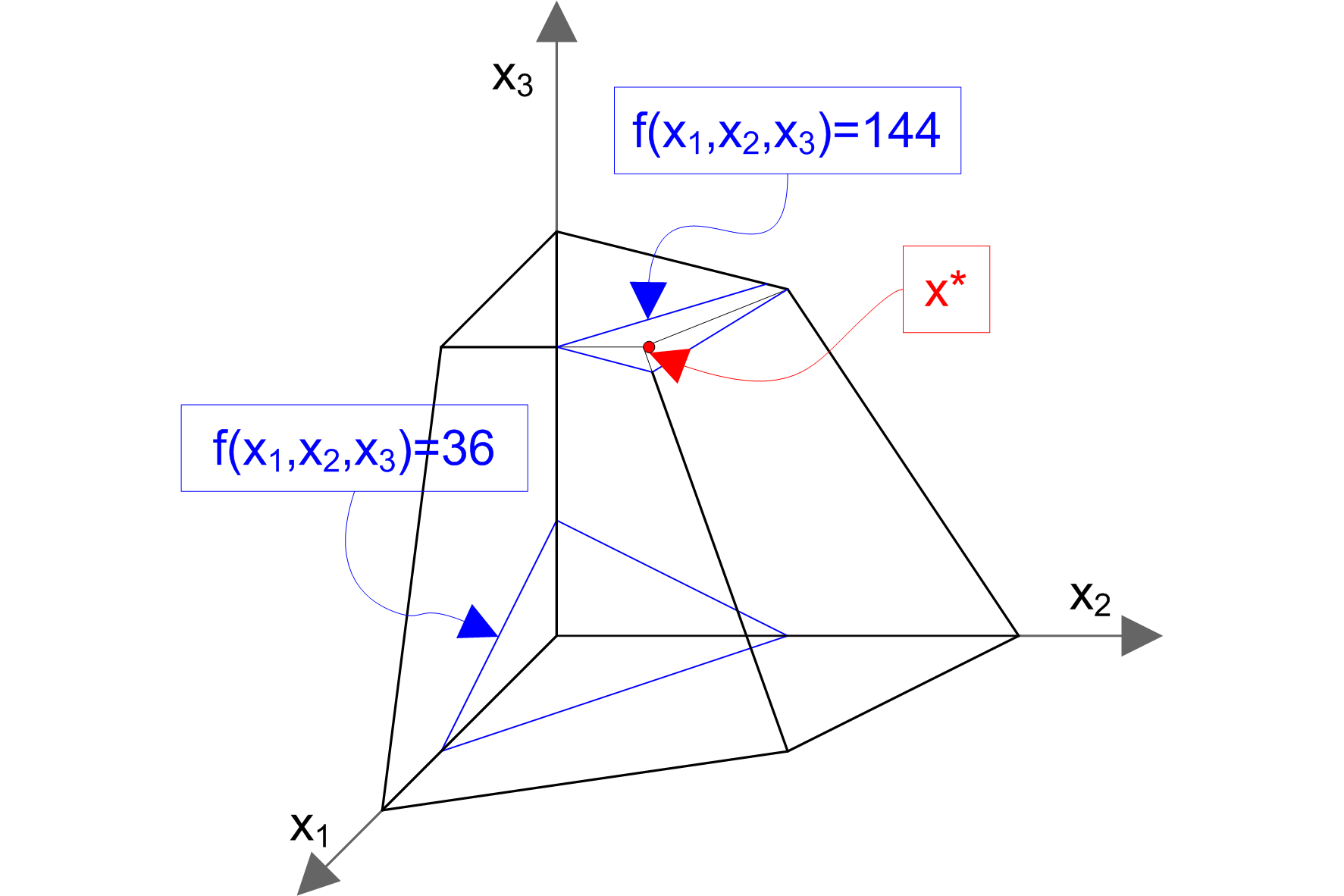
Zagadnienie trójwymiarowe
Model matematyczny zagadnienia:
max f(x) = 8*x1 + 9*x2 + 18*x3
15*x1 + 5*x2 + 6*x3
90
3*x1 + 6*x2 + 4*x3
48
x1 + x2 + 4*x3
28
x1
0, x2
0, x3
0
Optymalizacja w liczbach całkowitych
Zagadnienie wyznaczenia wartości optymalnej w liczbach całkowitych. Z przypadkiem takim można się spotkać w odniesieniu do dużych niepodzielnych obiektów typu samolotów, statków, turbin, zakładów produkcyjnych, w zagadnieniach transportu towarów.
Najprostszą metodą rozwiązania zagadnienia (dającą się zastosować wyjątkowo rzadko) może być zaokrąglenie do całkowitej wartości wyniku optymalizacji prowadzonej bez wymogu uzyskania wielkości całkowitych.
Większość pozostałych metod wymaga dwuetapowego procesu rozwiązania zagadnienia
etap pierwszy - wyznaczenie rozwiązania w liczbach ułamkowych,
etap drugi - sprowadzenie rozwiązania ułamkowego do rozwiązania w liczbach całkowitych.
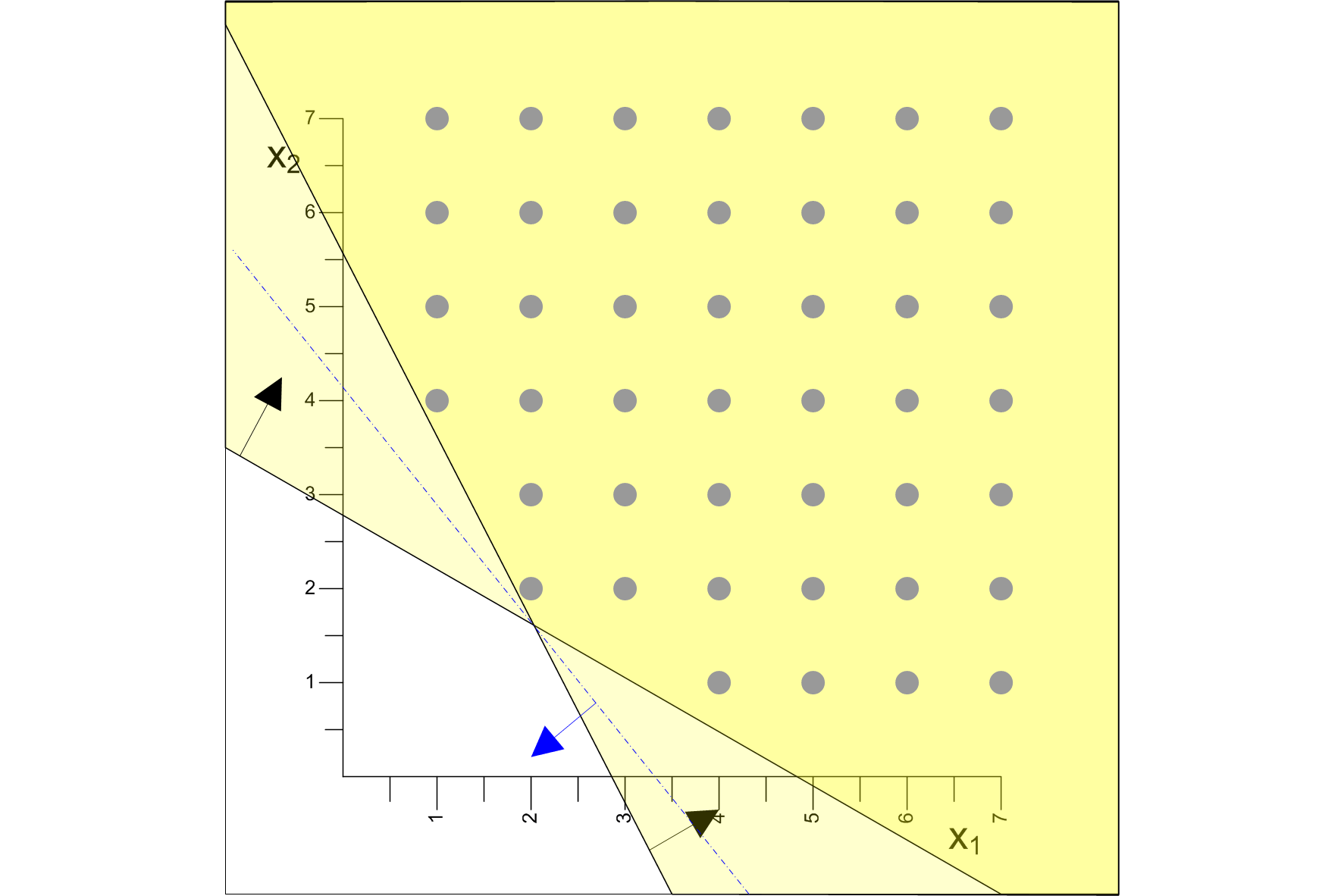
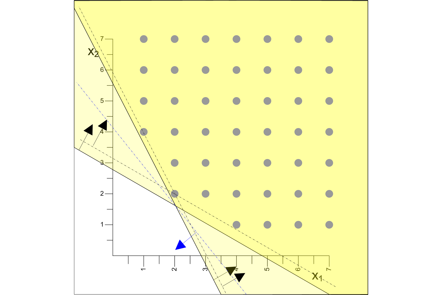
Optymalizacja w liczbach całkowitych
Metoda A.H.Landa-A.G.Doiga
etap pierwszy - wyznaczenie rozwiązania optymalnego w liczbach ułamkowych,
etap drugi - przejście do rozwiązania w liczbach całkowitych przez przesunięcie warstwicy optymalnej w głąb obszaru rozwiązań dopuszczalnych, aż do uzyskania pierwszego rozwiązania całkowitego. Przesunięcie wiąże się z uzyskaniem gorszej wartości funkcji kryterium.
Optymalizacja w liczbach
Metoda R.E.Gomory'ego całkowitych
etap pierwszy - wyznaczenie rozwiązania optymalnego w liczbach ułamkowych,
etap drugi - dodanie do warunków ograniczających nowego warunku (nowych warunków) oraz nowej zmiennej (nowych zmiennych) do zbioru zmiennych decyzyjnych.
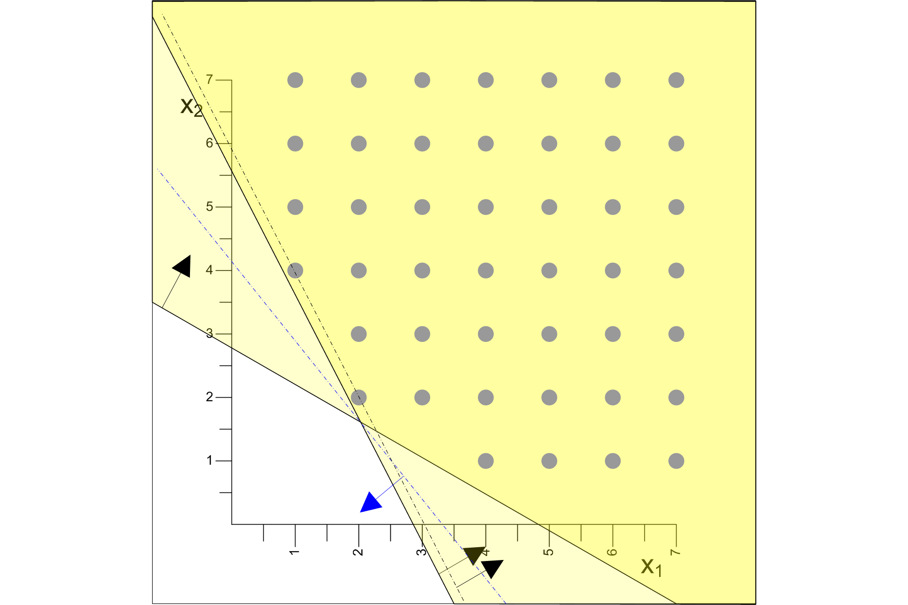
max f(x) = 6*x1 + 2.5*x2
x1
0
x2
0
9*x1 + 11*x2
99
12*x1 + 8*x2
96
x2
1
10*x1 + 10*x2
125
max f(x) = 6*x1 + 2.5*x2
x1
0
x2
0
9*x1 + 11*x2
99
12*x1 + 8*x2
96
x2
1
10*x1 + 10*x2
125
max f(x) = 6*x1 + 2.5*x2
x1
0
x2
0
9*x1 + 11*x2
99
12*x1 + 8*x2
96
x2
1
10*x1 + 10*x2
125
max f(x) = 6*x1 + 2.5*x2
x1
0
x2
0
9*x1 + 11*x2
99
12*x1 + 8*x2
96
x2
1
10*x1 + 10*x2
125
max f(x) = 6*x1 + 2.5*x2
x1
0
x2
0
9*x1 + 11*x2
99
12*x1 + 8*x2
96
x2
1
10*x1 + 10*x2
125
max f(x) = 6*x1 + 2.5*x2
x1
0
x2
0
9*x1 + 11*x2
99
12*x1 + 8*x2
96
x2
1
10*x1 + 10*x2
125
max f(x) = 6*x1 + 2.5*x2
x1
0
x2
0
9*x1 + 11*x2
99
12*x1 + 8*x2
96
x2
1
10*x1 + 10*x2
125
max f(x) = 6*x1 + 2.5*x2
x1
0
x2
0
9*x1 + 11*x2
99
12*x1 + 8*x2
96
x2
1
10*x1 + 10*x2
125
max f(x) = 6*x1 + 2.5*x2
x1
0
x2
0
9*x1 + 11*x2
99
12*x1 + 8*x2
96
x2
1
10*x1 + 10*x2
125
max f(x) = 6*x1 + 2.5*x2
x1
0
x2
0
9*x1 + 11*x2
99
12*x1 + 8*x2
96
x2
1
10*x1 + 10*x2
125
max f(x) = 6*x1 + 2.5*x2
x1
0
x2
0
9*x1 + 11*x2
99
12*x1 + 8*x2
96
x2
1
10*x1 + 10*x2
125
max f(x) = 6*x1 + 2.5*x2
x1
0
x2
0
9*x1 + 11*x2
99
12*x1 + 8*x2
96
x2
1
10*x1 + 10*x2
125
max f(x) = 6*x1 + 2.5*x2
x1
0
x2
0
9*x1 + 11*x2
99
12*x1 + 8*x2
96
x2
1
10*x1 + 10*x2
125
max f(x) = 6*x1 + 2.5*x2
x1
0
x2
0
9*x1 + 11*x2
99
12*x1 + 8*x2
96
x2
1
10*x1 + 10*x2
125
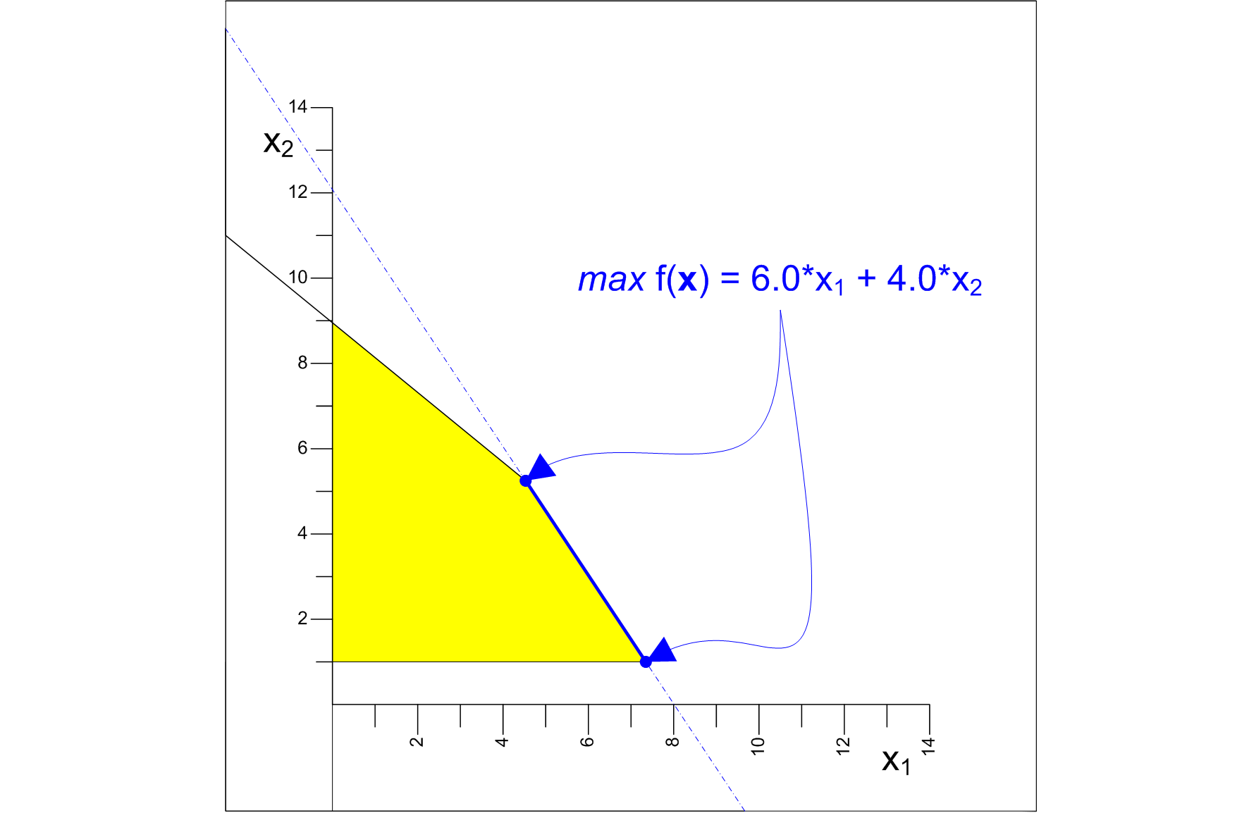
max f(x) = 6*x1 + 4.0*x2
x1
0
x2
0
9*x1 + 11*x2
99
12*x1 + 8*x2
96
x2
1
10*x1 + 10*x2
125
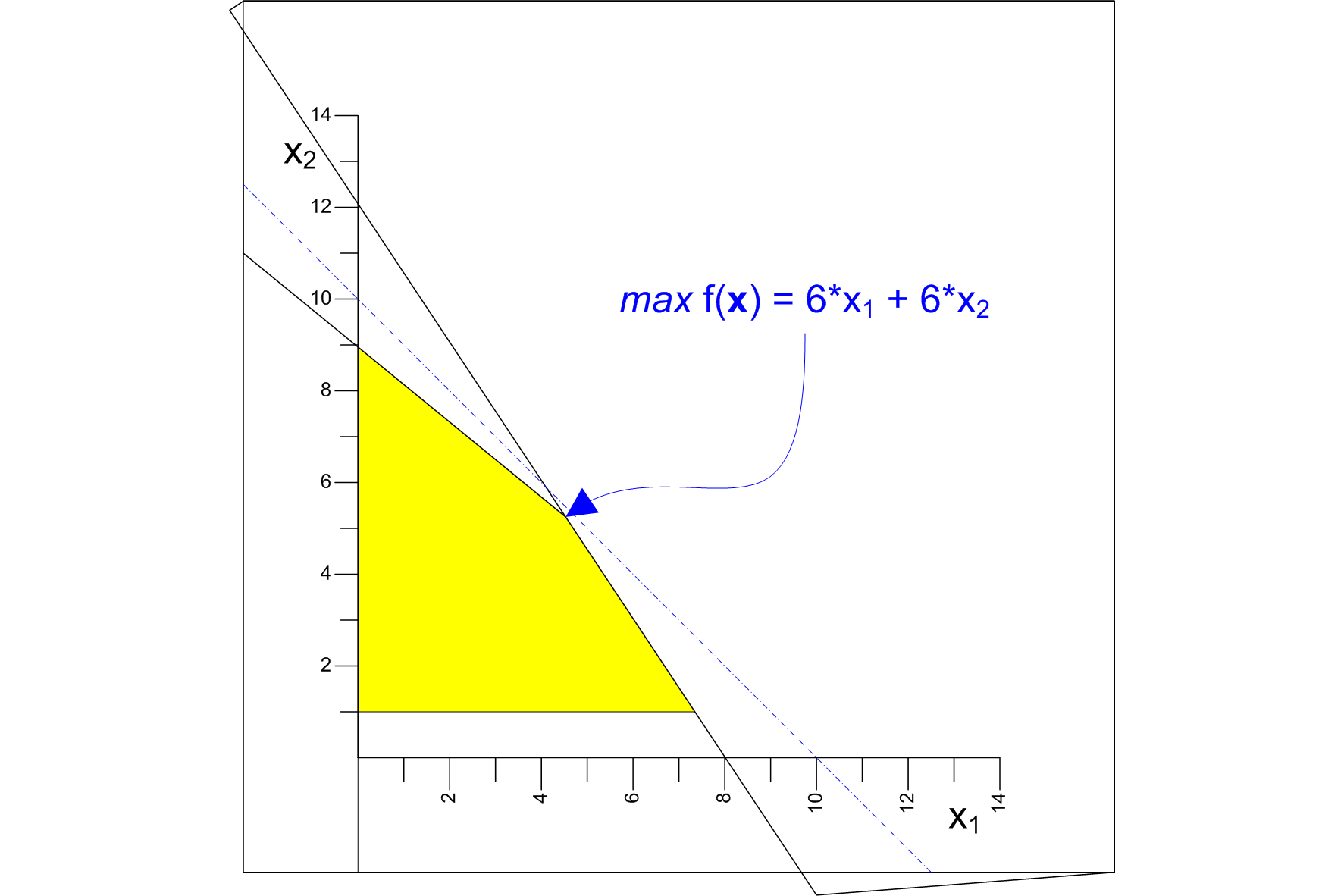
max f(x) = 6*x1 + 6.0*x2
x1
0
x2
0
9*x1 + 11*x2
99
12*x1 + 8*x2
96
x2
1
10*x1 + 10*x2
125
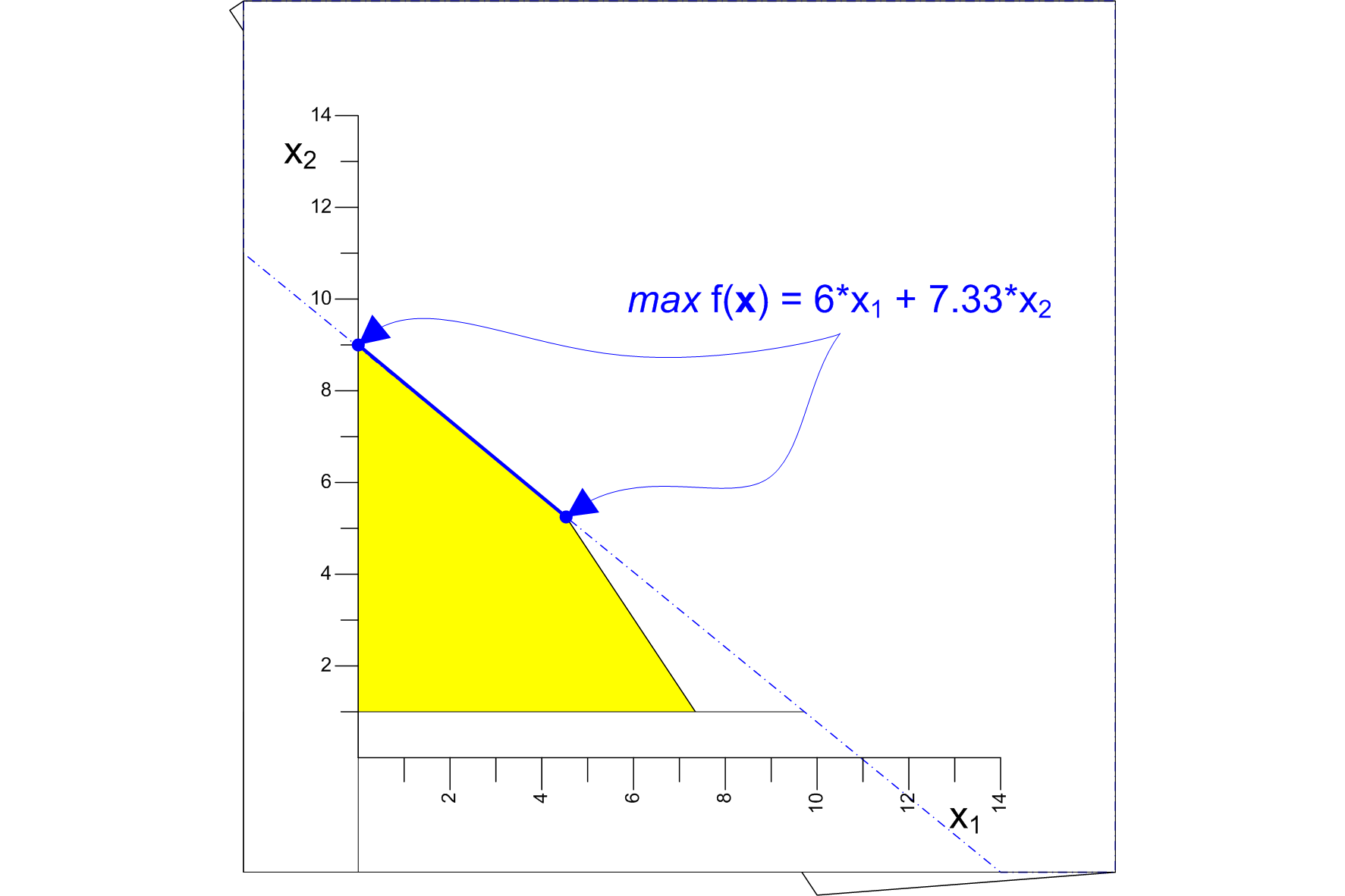
max f(x) = 6*x1 + 7.33*x2
x1
0
x2
0
9*x1 + 11*x2
99
12*x1 + 8*x2
96
x2
1
10*x1 + 10*x2
125
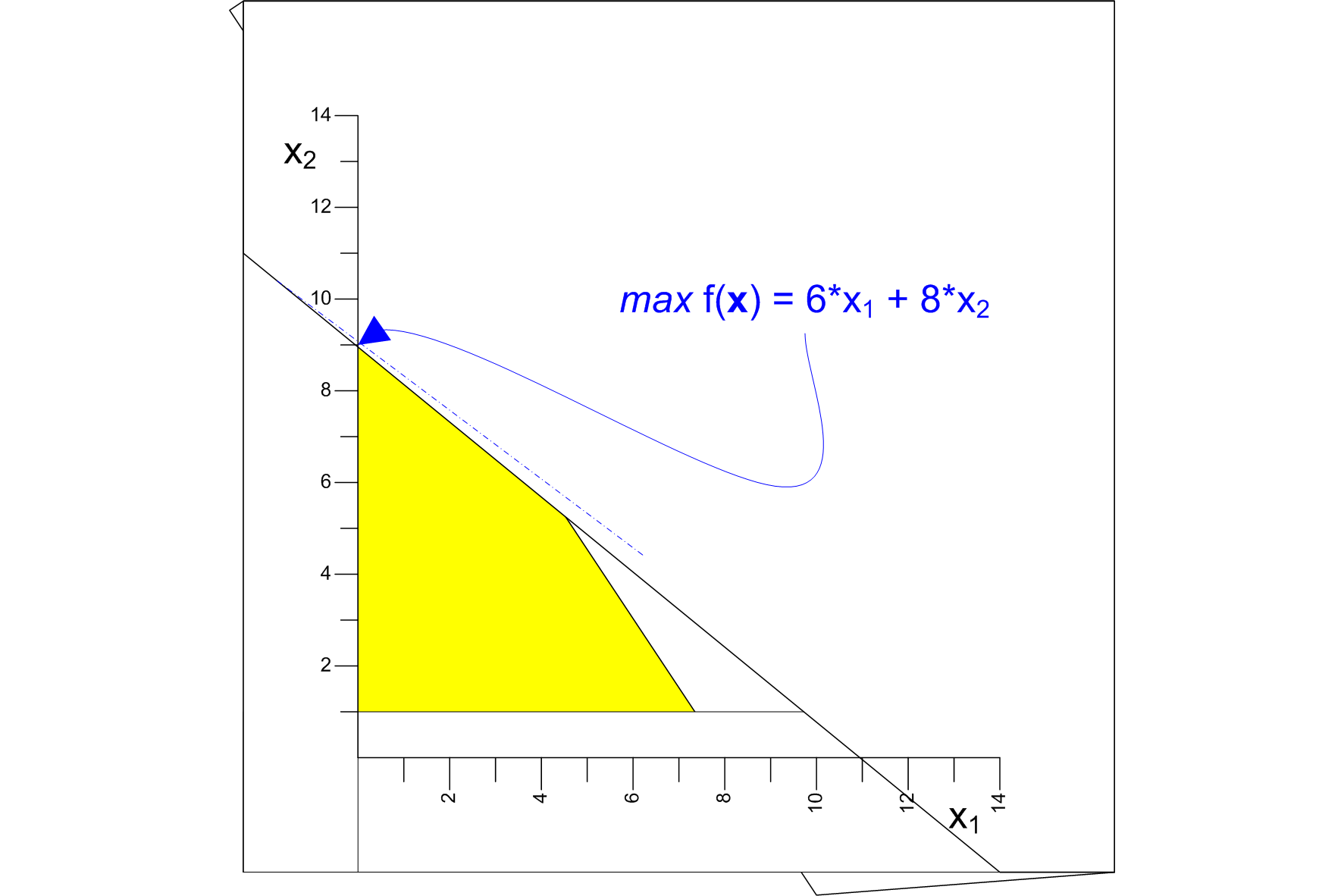
max f(x) = 6*x1 + 8.0*x2
x1
0
x2
0
9*x1 + 11*x2
99
12*x1 + 8*x2
96
x2
1
10*x1 + 10*x2
125
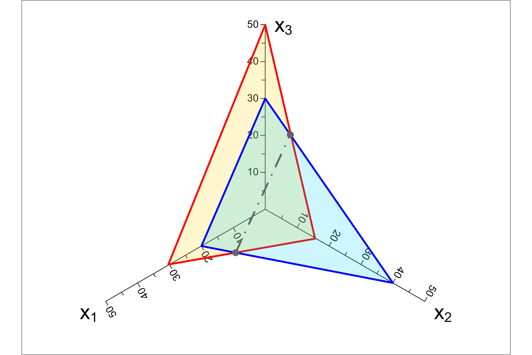
75*x1 + 150*x2 + 45*x3
2250
120*x1 + 60*x2 + 80*x3
2400
100*x1 + 40*x2 + 25*x3
1000
x1
0, x2
0, x3
0
75*x1 + 150*x2 + 45*x3
2250
120*x1 + 60*x2 + 80*x3
2400
100*x1 + 40*x2 + 25*x3
1000
x1
0, x2
0, x3
0
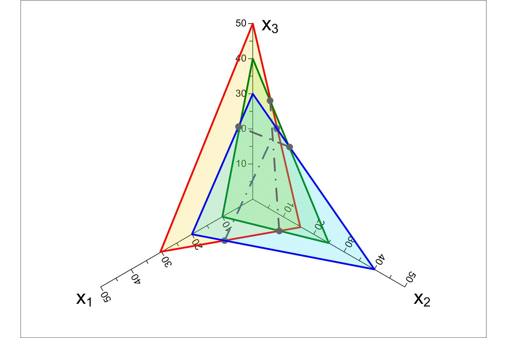
75*x1 + 150*x2 + 45*x3
2250
120*x1 + 60*x2 + 80*x3
2400
100*x1 + 40*x2 + 25*x3
1000
x1
0, x2
0, x3
0
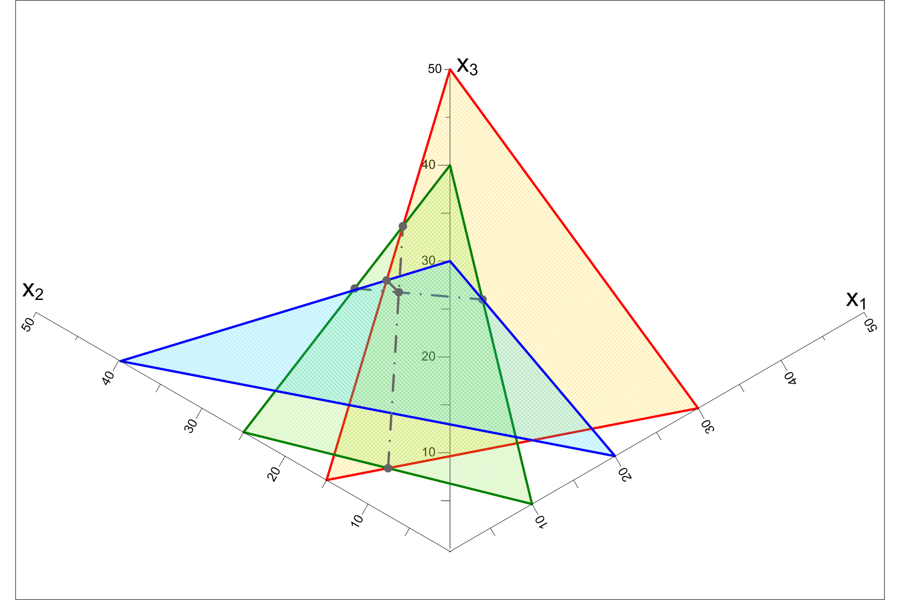
Wygląd obszaru dopuszczalnych rozwiązań od strony początku układu współrzędnych
75*x1 + 150*x2 + 45*x3
2250
120*x1 + 60*x2 + 80*x3
2400
100*x1 + 40*x2 + 25*x3
1000
x1
0, x2
0, x3
0
max f(x) = 8*x1 + 9*x2 + 18*
15*x1 + 5*x2 + 6*x3
90
3*x1 + 6*x2 + 4*x3
48
x1 + x2 + 4*x3
28
x1
0, x2
0, x3
0
Wyszukiwarka
Podobne podstrony:
wykład 1 Rybinski
wykład 4 Rybiński
wykład 2 Rybinski
Napęd Elektryczny wykład
wykład5
Psychologia wykład 1 Stres i radzenie sobie z nim zjazd B
Wykład 04
geriatria p pokarmowy wyklad materialy
ostre stany w alergologii wyklad 2003
WYKŁAD VII
Wykład 1, WPŁYW ŻYWIENIA NA ZDROWIE W RÓŻNYCH ETAPACH ŻYCIA CZŁOWIEKA
Zaburzenia nerwicowe wyklad
Szkol Wykład do Or
Strategie marketingowe prezentacje wykład
Wykład 6 2009 Użytkowanie obiektu
wyklad2
wykład 3
więcej podobnych podstron