Wykład 7

Przyśpieszenie dowolnego punktu B pręta AB poruszającego się ruchem płaskim, jest równe sumie geometrycznej przyśpieszenia dowolnie obranego punktu A oraz przyśpieszenia punktu B wynikającego z obrotu względem punktu A.

Ruch kulisty ciała sztywnego

Ruchem kulistym ciała sztywnego nazywamy taki ruch ciała podczas którego jeden jego punkt pozostaje nieruchomy

ξ - ksi, ψ - psi, ζ - dzeta, φ - fi, η - eta,
- teta

Układ nieruchomy 0xyz, wersory tego układu i₁, j₁, k₁,

układ związany z ciałem 0ξηζ, wersory tego układu i₂, j₂, k₂

ζ z Patrz Jan Misiak tom II

η strona 105

M

r z

0 y ζ

x ξ k₁ η

k₂

0 y

ψ

ω x

k₃ φ ξ

M^' n

*r *θ

M ψ, φ,
- kąty Eulera

r

*θ Rys.54 Obrót ciała

0

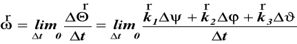
Wektor wypadkowy małego obrotu *θ jest równy

sumie geometrycznej wektorów małych obrotów wokół poszczególnych osi

(70)

Prędkości kątowe i liniowe w ruchu kulistym

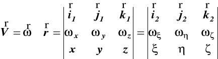
Prędkość liniowa punktu M (rys.54)jest równa

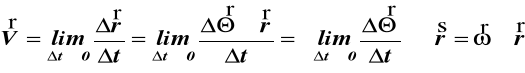
(71)

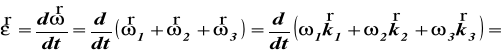
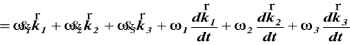
gdzie ω - chwilowa prędkość kątowa ciała sztywnego

(72)

ω₁ -prędkość kątowa precesji, wektor ω₁ pokrywa się z 0z

ω₂- prędkość kątowa obrotu własnego, wektor ω₂ pokrywa

się z osią układu ruchomego 0 ζ

ω₃- prędkość kątowa nutacji, wektor ω₃ leży na linii węzłów

0n (rys.54)

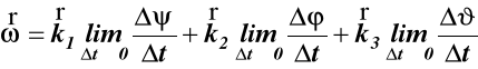
Składowe wektora prędkości kątowej ω :

(73)

(74)

47a.kin

Rysunki do wzorów (73)

ζ z

ω₂cos

ω₂ ω₁ η

ω₂sin
cosΨ

ω₂sin
0 y 0 y

ψ ω₂sin

m ω₂sin
sinΨ

ω₃ ϕ ξ Ψ

x n m 90⁰-Ψ n

x

0 ω₃sinΨ

y

ω₃

m ω₃cosΨ

n

x

Rys.54a

47b.kin

Rysunki do wzorów (74)

z

ζ ω₁ η

π

ω

₁cosϑ

ω₂ π₁

n₁

ω₁sinϑ

ω₃ ξ

ϕ

n n jest prostopadłe do pł. π

a więc jest prostopadłe do n₁

n₁ jest prostopadłe do ζ bo

leży w pł. 0ξη

0 ω₁sinϑcosϕ

η

ω₁sinϑ

ϕ

ω₁sinϑsinϕ

n n₁

ξ

Rys.54b

ω₃sinϕ 0 η

ω₃ ω₃cosϕ

ϕ

n ξ

Znając położenie chwilowej osi obrotu i składowe

prędkości kątowej ciała wokół tej osi, można wyznaczyć prędkość liniową dowolnego punktu M ciała

(75)

Wartość liczbowa tej prędkości wynosi

(76)

z M

V

h

l

0 y

z x

x y Rys.55

Składowe prędkości liniowej punktu M w:

nieruchomym układzie współrzędnych 0xyz są równe

,
,

ruchomym układzie współrzędnych
wynoszą

,
,

Przyśpieszenie kątowe i liniowe w ruchu kulistym

Różniczkując (72) otrzymujemy przyśpieszenie kątowe

(77)

gdzie

Różniczkując (75) otrzymujemy wzór na

przyśpieszenie liniowe punktu M

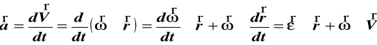
(78)

Chwilowe osie obrotu w układzie ruchomym tworzą pewną powierzchnię stożkową z wierzchołkiem w punkcie 0.

Aksoida ruchoma jest to miejsce geometryczne chwilowych osi obrotu w układzie ruchomym.

Aksoida nieruchoma jest to miejsce geometryczne chwilowych osi obrotu w układzie nieruchomym.

PRECESJA REGULARNA

Kąt precesji
= const, stąd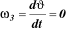

oraz ω₁ = const, ω₂ = const

l₀ z

ζ

υ

ω

ω₁ η

ω₂

0 y

x ψ ε ϕ ξ

n

Rys.56 Precesja regularna

Na podstawie wzoru (77) przyśpieszenie kątowe

(79)

Biorąc pod uwagę, że
otrzymamy

gdyż

Wektor przyśpieszenia kątowego ε o przyjętym początku w środku ruchu kulistego 0 jest prostopadły do wektorów

ω₁ i ω₂, a więc jest skierowany wzdłuż linii węzłów 0n

Przyśpieszenie liniowe a jest równe sumie geometrycznej przyśpieszenia precesyjnego a₁

(80)

i przyśpieszenia doosiowego a₂

(81)

(82)

Przykład 18

Stożek kołowy o kącie wierzchołkowym 2α = 60⁰ i długości tworzącej ściany bocznej l toczy się bez poślizgu po poziomej płaszczyźnie. Oś stożka obraca się ze stałą prędkością kątową precesji ω₁ s^-1 wokół pionowej osi 0z.

Obliczyć prędkości i przyśpieszenia liniowe punktów A i B.

z A

r_A

ω₁ 2α

B

ω y

0 r_B

ω₂

x

Rys.57

Rozwiązanie

Po przyjęciu w punkcie 0 nieruchomego układu współrzędnych 0xyz promienie wektory punktów A i B wynoszą:

,

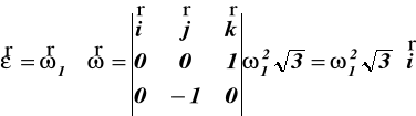
Prędkości kątowe są równe

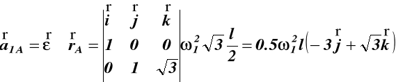
Z wzoru (75) określamy prędkości:

dla punktu A

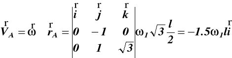
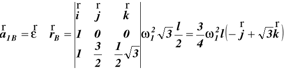
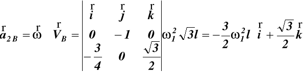
dla punktu B

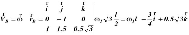
Przyśpieszenie kątowe
stożka wyznaczamy ze wzoru (79)

Przyśpieszenia liniowe punktów A i B z wzorów (80*82) wynoszą:

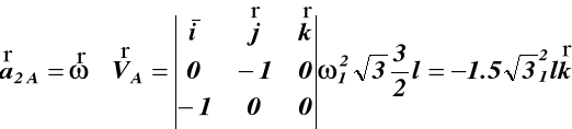
a_Bx

a_B

a_By B y

i j

x

Rys.58

46kin

47kin

48kin

r

α

ω

49kin

50kin

51kin

52kin

---